Drug repositioning (also called drug repurposing) involves the investigation of existing drugs for new therapeutic purposes. Through graph analytics and machine learning applied to knowledge graphs, drug repurposing aims to find new uses for already existing and approved drugs. This approach, part of a more general science called in-silico drug discovery, makes it possible to identify serious repurposing candidates by finding genes involved in a specific disease and checking if they interact, in the cell, with other genes which are targets of known drugs The discovery of new treatments through drug repositioning complements traditional drug development for small markets that include rare diseases. It involves the identification of single or combinations of existing drugs based on human genetics data and network biology approaches represents a next-generation approach that has the potential to increase the speed of drug discovery at a lower cost.

In this article we show in details how a freely available but real-world biomedical knowledge graph (the Drug Repurposing Knowledge Graph or DRKG) can generate compounds for concrete diseases. As an example, we show how to discover new compounds to treat hypertension (high blood pressure). We use TigerGraph as a backend graph database to store the knowledge graph and the newly discovered relationships together with some graph machine learning techniques (in easy to use Python frameworks).

From a bird’s eye view:

  • DRKG: an overview of what the knowledge contains
  • TigerGraph schema: how to connect and define a schema for the knowledge graph
  • Querying: how to use the TigerGraph API from Python
  • Data import: how import the TSV data into TigerGraph
  • Exploration and visualization: what does the graph look like?
  • Link prediction: some remarks on how one can predict things without neural networks
  • Drug repurposing the hard way: possible paths and frameworks
  • Drug repurposing the easy way: TorchDrug and pretrained vectors to the rescue
  • Repurposing for hypertension: concrete code to make the world a better place
  • Challenges: some thoughts and downsides to the method
  • References: links to books, articles and frameworks
  • Setup: we highlight the necessary tech you need to make it happen

You will also find a list of references and your feedback is always welcome via Twitter, via the Github repo or via Orbifold Consulting.

With some special thanks to Cayley Wetzig for igniting this article.

Drug Repurposing Knowledge Graph (DRKG)

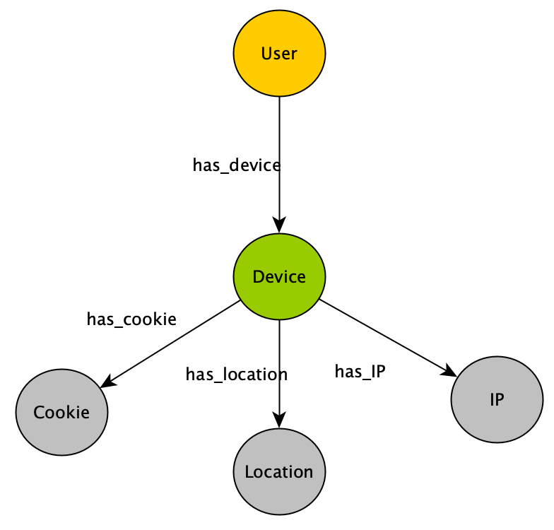
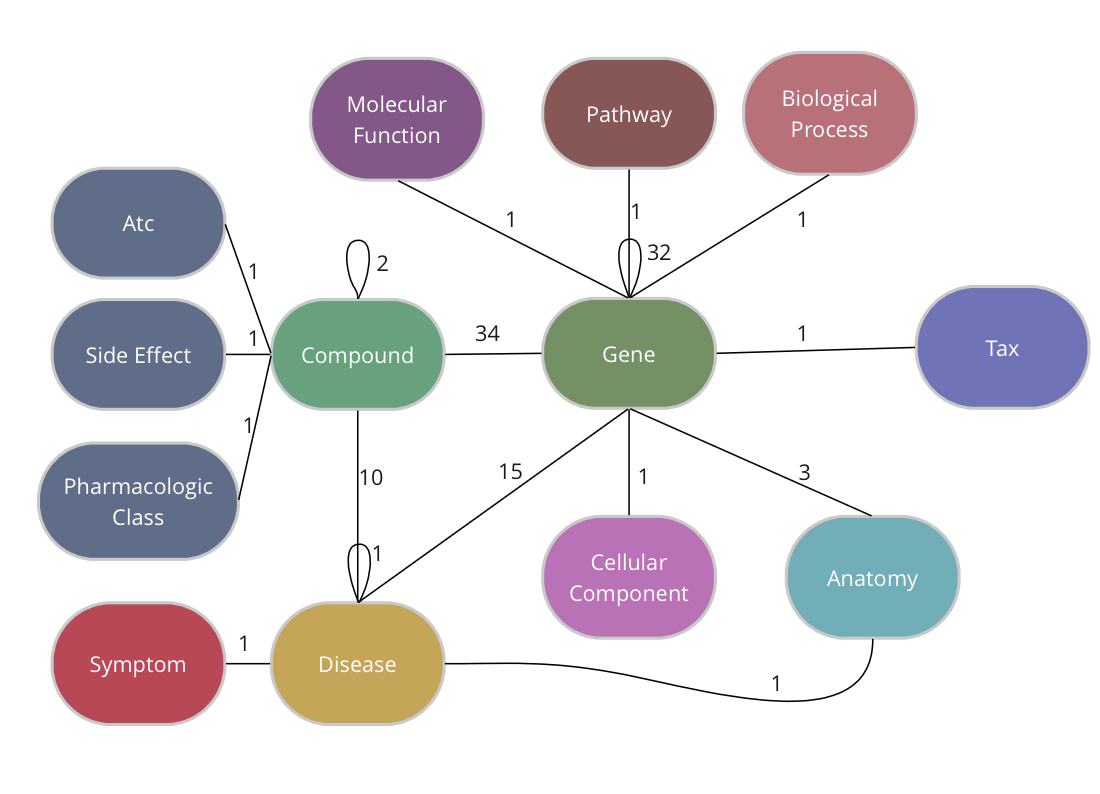
The Drug Repurposing Knowledge Graph (DRKG) is a comprehensive biological knowledge graph relating genes, compounds, diseases, biological processes, side effects and symptoms. DRKG includes information from six existing databases (DrugBank, Hetionet, GNBR, String, IntAct and DGIdb) as well as data collected from recent publications, particularly related to Covid19. It includes 97,238 entities belonging to 13 entity-types; and 5,874,261 triplets belonging to 107 edge-types. These 107 edge-types show a type of interaction between one of the 17 entity-type pairs (multiple types of interactions are possible between the same entity-pair), as depicted in the adjacent image.

The DRKG data is freely available we explain below how you can import the data into TigerGraph.

Creating the schema in TigerGraph

TigerGraph has an integrated schema designer which allows one to design a schema with ease. There is also an API to define a schema via code and since the DRKG schema has lots of edge types between some entities (Compound-Gene has 34, Gene-Gene has 32), it’s easier to do it via code. The method below, in fact, allows you to output a schema for any given dataset of triples.

The end-result inside TigerGraph can be seen in the adjacent picture and is identical to the schema above. The many reflexive edges you see are an explicit depiction of the multiple edge count above.

Generating the schema involves the following elements:

  1. given the triples collection, we loop over each one to harvest the endpoints (aka head and tail) and name of the relation (aka relation or predicate)
  2. the endpoints are in the form “type::id” so we split the string to extract the type and the id
  3. each node type and node id are bundled in entity collection
  4. the names of the relations are cleaned and put in a separate dictionary.

A typical relation name (e.g. “DRUGBANK::ddi-interactor-in::Compound:Compound”) contains some special characters which are not allowed in a TigerGraph schema. All of these characters are removed but this is the only difference with the initial (raw) data.

Once you have downloaded the dataset you should see a TSV file called “drkg.tsv”. This contains all the triples (head-relation-tail) and it can be loaded with a simple Pandas method:

import pandas as pd
drkg_file = './drkg.tsv'
df = pd.read_csv(drkg_file, sep="\t")
triplets = df.values.tolist()

The triplets list is a large array of 5874260 items.

Next, the recipe above output a string which one can execute inside TigerGraph; a schema creation query.

rtypes = dict() # edge types per entity-couple
entity_dic = {} # entities organized per type
for triplet in triplets:
    [h,r,t] = triplet
    h_type = h.split("::")[0].replace(" " ,"")
    h_id = str(h.split("::")[1])
    t_type = t.split("::")[0].replace(" " ,"")
    t_id = str(t.split("::")[1])

    # add the type if not present
    if not h_type in entity_dic:
        entity_dic[h_type]={}
    if not t_type in entity_dic:
        entity_dic[t_type] ={}

    # add the edge type per type couple
    type_edge = f"{h_type}::{t_type}"
    if not type_edge in rtypes:
        rtypes[type_edge]=[]
    r = r.replace(" ","").replace(":","").replace("+","").replace(">","").replace("-","")
    if not r in rtypes[type_edge]:
        rtypes[type_edge].append(r)

    # spread entities
    if not h_id in entity_dic[h_type]:
        entity_dic[h_type][h_id] = h
    if not t in entity_dic[t_type]:
        entity_dic[t_type][t_id] = t

schema = ""
for entity_type in entity_dic.keys():
    schema += f"CREATE VERTEX {entity_type} (PRIMARY_ID Id STRING) With primary_id_as_attribute=\"true\"\n"
for endpoints in rtypes:
    [source_name, target_name] = endpoints.split("::")
    for edge_name in rtypes[endpoints]:
        schema += f"CREATE DIRECTED EDGE {edge_name} (FROM {source_name}, TO {target_name})\n"
print(schema)

TigerGraph has excellent documentation and you should read through the “Defining a graph schema” topic which explains in detail the syntax used in the script above.

The output of this Python snippet (full listing here) looks like the following

CREATE VERTEX Gene (PRIMARY_ID Id STRING) With primary_id_as_attribute="true"
CREATE VERTEX Compound (PRIMARY_ID Id STRING) With primary_id_as_attribute="true"
...
CREATE DIRECTED EDGE GNBRZCompoundGene (FROM Compound, TO Gene)
CREATE DIRECTED EDGE HetionetCbGCompoundGene (FROM Compound, TO Gene)
...

You can use this directly in a GSQL interactive session or via one of the many supported languages. As described in the next section, we’ll use Python with the pyTigerGraph driver to push the schema.

Connecting and querying

Obviously, you need a TigerGraph instance somewhere and if you don’t have one around there is no easier way than via the TigerGraph Cloud.

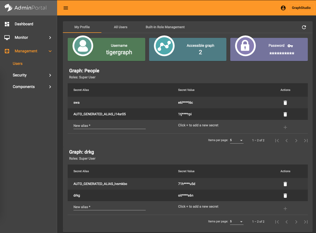
In the AdminPortal (see image) you should add a secret specific to the database. That is, you can’t use a global secret to connect, you need one per database.

Installing the pyTigerGraph drive/package is straightforward (pip install pyTigerGraph) and connecting to the database with the secret looks like the following:

import pyTigerGraph as tg
host = 'https://your-organization.i.tgcloud.io'
secret = "your-secret"
graph_name = "drkg"
user_name = "tigergraph"
password = "your-password"
token = tg.TigerGraphConnection(host=host, graphname=graph_name, username=user_name, password=password).getToken(secret, "1000000")[0]
conn = tg.TigerGraphConnection(host=host, graphname=graph_name, username=user_name, password=password, apiToken=token)

This can be condensed to just three lines but the explicit naming of the parameters is to help you get it right.

If all is well you can test the connection with

conn.echo()

which returns “Hello GSQL”. With this connection you can now use the full breadth of the GSQL query language.

In particular, we can now create the schema assembled above with this:

print(conn.gsql(
"""
    use global
    CREATE VERTEX Gene (PRIMARY_ID Id STRING) With primary_id_as_attribute="true"
    CREATE VERTEX Compound (PRIMARY_ID Id STRING) With primary_id_as_attribute="true"
    ...
    CREATE DIRECTED EDGE GNBRZCompoundGene (FROM Compound, TO Gene)
    CREATE DIRECTED EDGE HetionetCbGCompoundGene (FROM Compound, TO Gene)
...
""")

The content is a copy of the outputted string plus an extra statement use global to generate the schema in the global TigerGraph namespace. It means that the schema elements can be reused across different databases. This feature is something you will not find in any other graph database solution and has far-reaching possibilities to manage data.

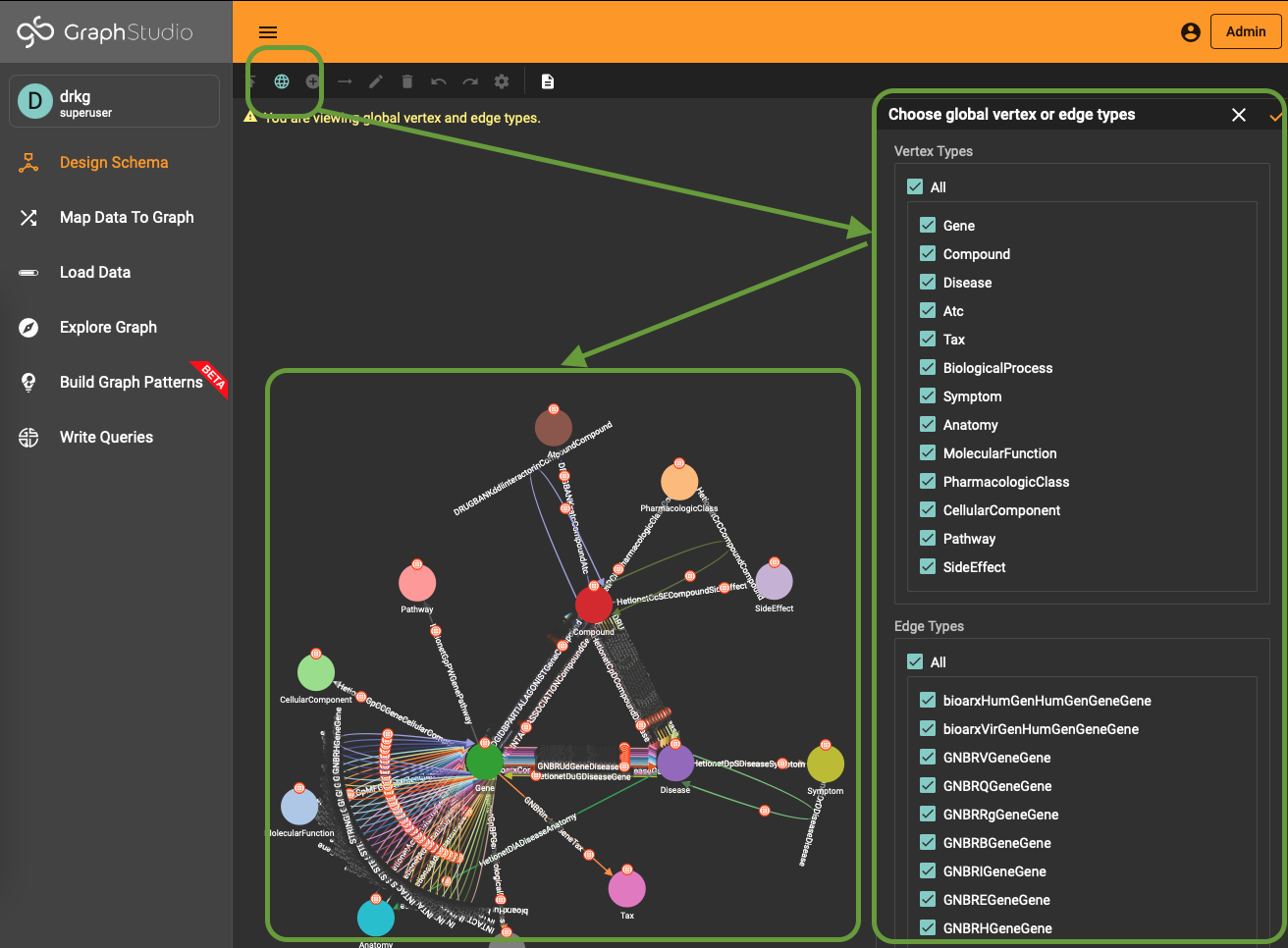
To use (part of) the global schema in a specific database you simply have to go into the database schema designer and import the elements from the global schema (see picture). Note that in the visualization you have a globe-icon to emphasize that a schema element is inherited from the global schema.

Importing the data

The Jupyter notebook to create the schema as well as to import the data can be found here.

TigerGraph has a wonderful intuitive interface to import data but the DRKG schema contains a lot of loops and the raw TSV has the node type embedded in the triple endpoints. One approach is to develop some ETL to end up with multiple files for each entity type and the relationships. The easier way is to use the REST interface to the database:

for triplet in triplets:
    [h,r,t] = triplet
    h_type = h.split("::")[0].replace(" " ,"")
    h_id = str(h.split("::")[1])
    t_type = t.split("::")[0].replace(" " ,"")
    t_id = str(t.split("::")[1])
    r = r.replace(" ","").replace(":","").replace("+","").replace(">","").replace("-","")

    conn.upsertEdge(h_type, h_id, r, t_type, t_id)

The upsertEdge method also creates the nodes if they are not present already, there is no need to upsert nodes and edges separately. This approach is much easier than the ETL one but the hidden cost is the fact that it engenders 5.8 million REST calls. In any case, creating such a large graph takes time no matter the approach.

If you are only interested in exploring things or you have limited resources, you can sample the graph and create a subgraph of DRKG fitting your needs:

amount_of_edges = 50000
triple_count = len(triplets)
sample = np.random.choice(np.arange(triple_count), amount_of_edges)
for i in sample:
    [h,r,t] = triplet
    h_type = h.split("::")[0].replace(" " ,"")
    h_id = str(h.split("::")[1])
    t_type = t.split("::")[0].replace(" " ,"")
    t_id = str(t.split("::")[1])
    r = r.replace(" ","").replace(":","").replace("+","").replace(">","").replace("-","")

    conn.upsertEdge(h_type, h_id, r, t_type, t_id)

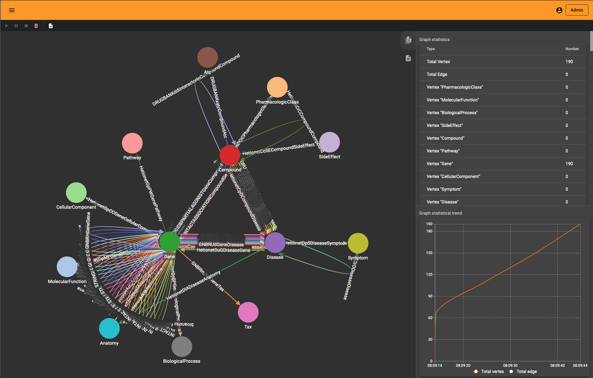
One neat thing you’ll notice is that “Load Data” interface in TigerGraph Studio also shows the import progress if you use the REST API. You see the graph growing (to the entity and edge type level) whether you use the ETL upload or the REST import.

Exploration and Visualization

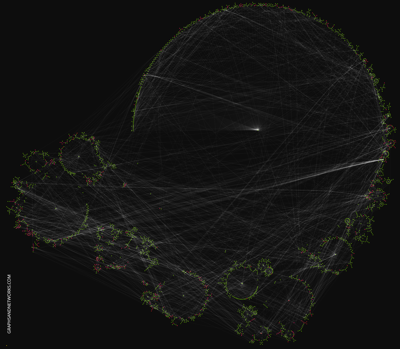
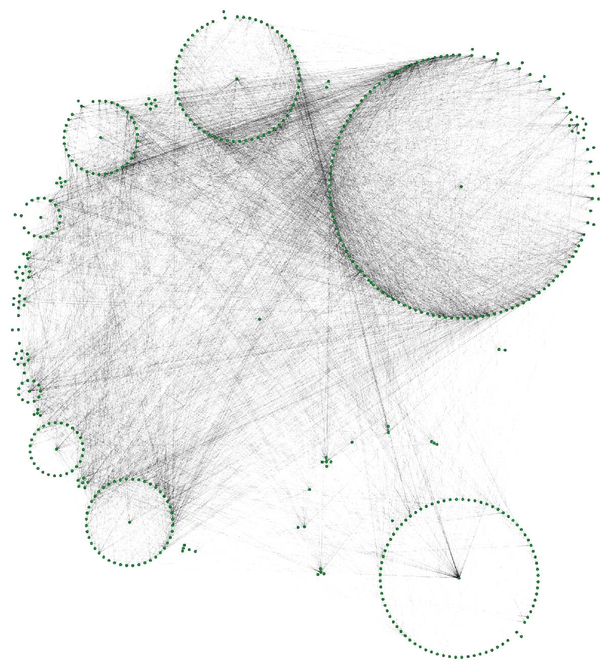
If you wonder how the DRKG graph looks like, the 0.01 ratio of node to edges automatically leads to a so-called hairball. The degree histogram confirms this and like many real-world graphs it exhibits a power-law distribution (aka scale-free network), meaning that the connectivity is mostly defined through a small set of large hubs while the mjority of the nodes has a much smaller degree.

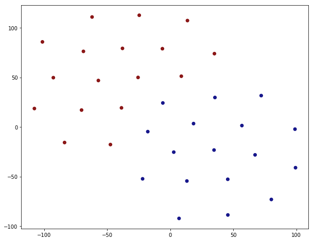
To layout the whole graph you can use for instance the wonderful Rapids library and the force-atlas algorithm or Gephi but you will need some patience and the result will look like the image below.

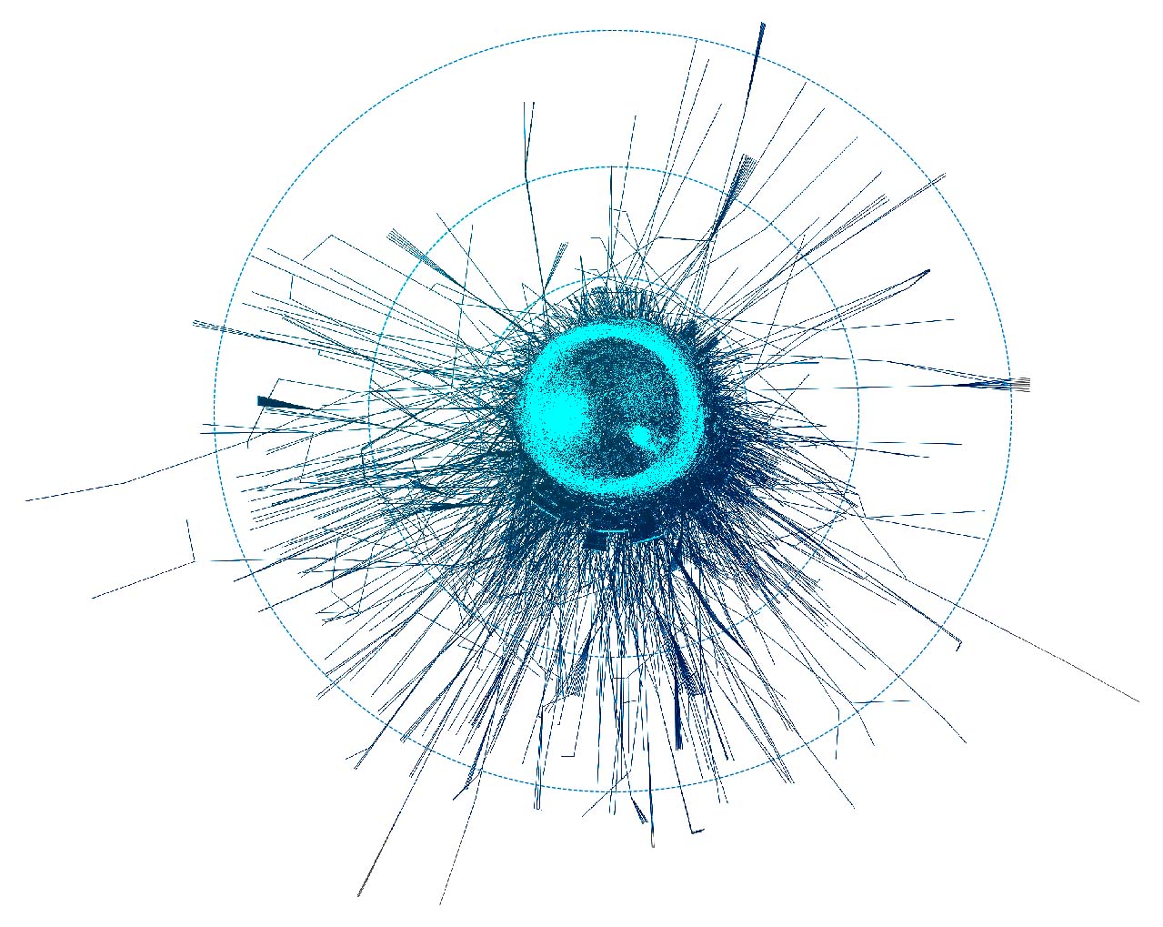
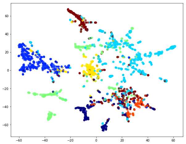
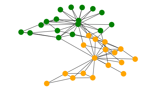
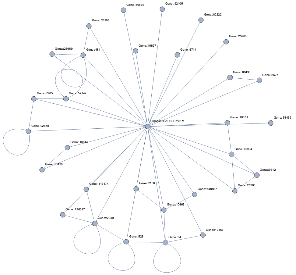
Taking a subset of the whole graph reveals something more pleasing and if you hand it over to yEd Live you’ll get something like the following

DRKG Visualization

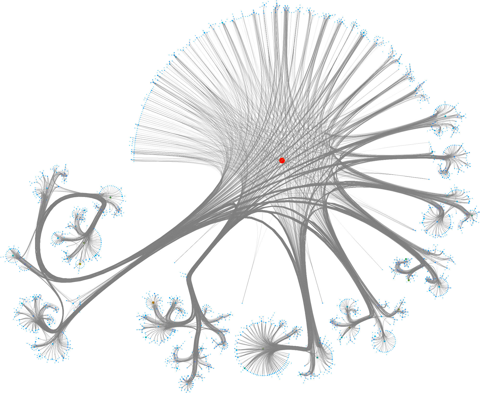
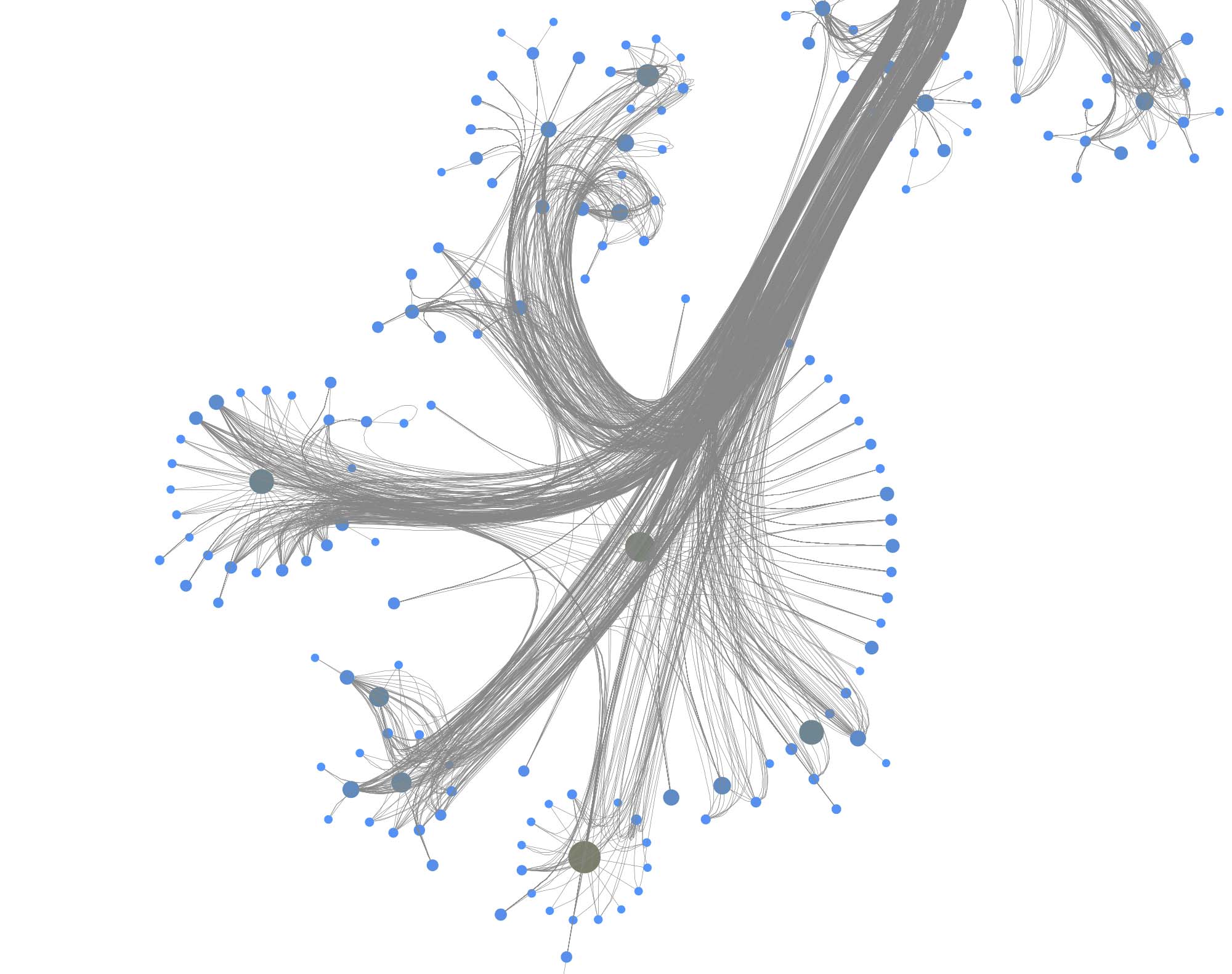
You can furthermore use degree centrality (or any other centrality measure) to emphasize things and zooming into some of the clusters you can discover gene interactions or particular disease symptoms. Of course, all of this is just exploratory but just like any other machine learning task it’s crucial to understand a dataset and gain some intuition.

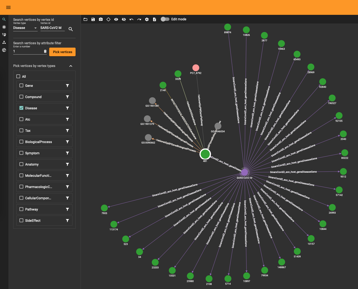
The DRKG data contains interesting information about COVID (variations). For example, the identifier “Disease::SARS-CoV2 M” refers to “severe acute respiratory syndrome coronavirus 2 membrane (M) protein” and you can use a simple GSQL query

CREATE QUERY get_covid() FOR GRAPH drkg {

    start =   {Disease.*};
    results = SELECT s FROM start:s WHERE s.id=="SARS-CoV2 M";
    PRINT results;

}

to fetch the data or use the TigerGraph data explorer. The data explorer having the advantage that you can dril down and use various layout algorithms on the fly.

Topological Link Predictions

With all the data in the graph database you can start exploring the graph. The TigerGraph GraphStudio offers various click-and-run methods to find shortest paths and other interesting insights. At the same time, the Graph Data Science Library (GDSL) has plenty of methods you can run to discover topological and other characteristics. For example, there are 303 (weakly) connected components and the largest one contains 96420 nodes while the rest are tiny islands of less than 30 nodes. This means that the gross of the data sits in the main component (consisting of 4400229 edges). You can obtain this info using GDSL using the query RUN QUERY tg_conn_comp(...) .

In the same fashion you can run GDSL methods to fetch the k-cores, the page rank and many other standard graph analytical insights. There is also a category entitled “Topological Link Prediction” and although it does what it says it’s often not sufficient to for graph completion purposes. There are various reasons for this:

  • the word “topological” refers here to the fact that the computation only takes the connectivity into account, not the potential data contained in a node or the payload on an edge. Althoug the DRKG does not have rich data inside the nodes and edges, in general one has molecular information (chemical properties), disease classes and so on. This data is in many cases at least as important as the topological one and to accurately predict new edges (or any other ML task) this data has to be included in the prediction pipeline.
  • algorithms like the Jaccard similarity only goes one level deep in searching for similarities. Of course, this has to do with algorithmic efficiency since looping over more than 5 million edges and vertex neighborhoods is demanding. In general, however, the way a node is embedded in a graph requires more than the immediate children/parents of the node.
  • topological link prediction does not infer the edge type or other data, only that an edge ‘should’ be present in a statistical sense.

At the same time one can question how meaningful it is to implement more advanced machine learning (i.e. neural networks and alike) on a database level. This remark is valid for any database, not just TigerGraph. Whether you use StarDog, SQL Server or Neo4j there some issues with embedding machine learning algorithms in a database:

  • training neural networks without the raw power of GPU processing is only possible for small datasets. Embedding graph machine learning in a database implicitly requires a way to integrate Nvidia somewhere.
  • whether you need Spark or Dask (or any other distributed processing magic) to get the job done, it leads to a whole lot of packages and requirements. Not mentioning the need to have virtual environments and all that.
  • feature engineering matters and when transforming a graph to another one (or turning it into some tabular/numpy format) you need to store things somewhere. Neo4j for example uses projections (virtual graphs) but it’s not a satisfactory solution (one cannot query projections for one).
  • there are so many ML algorithms and packages out there that it’s hardly possible to consolidate something which will answer to all business needs and graph ML tasks.

This is only to highlight that any data science library within a graph database (query language) has its limitations and that one inevitably needs to resort to a complementary solution outside the database. A typical enterprise architecture with streaming data would entail things like Apache Kafka, Amazon Kinesis, Apache Spark and all that. The general idea is as follows:

  • a representative subgraph of the graph database is extracted in function of machine learning
  • a model is trained towars the (business) goal: graph classification, link prediction, node tagging and so on
  • the model is used outside the graph database (triggered upon new graph data) and returns some new insight
  • the insight is integrated into the original graph.

In practice this involves a lot of work and some tricky questions (e.g. how to make sure updates don’t trigger the creation of existing edges) but the crux is that like so often a system should be used for what it’s made for.

With respect to drug repurposing using the DRKG graph, altough GSQL is Turing complete and hence in theory capable of running neural networks we will assemble in the next section a pipeline outside TigerGraph and feed the new insights back via a simple upsert thereafter.

Drug repurposing using Geometric Deep Learning

Graph machine learning is a set of techniques towards various graph-related tasks, to name a few:

  • graph classification: assigning a label to a while graph. For instance, determining whether a molecule (seen as a graph) is toxic or not.
  • node classification: assigning a label to a given node. For instance, inferring the gender in a social network based on given attributes.
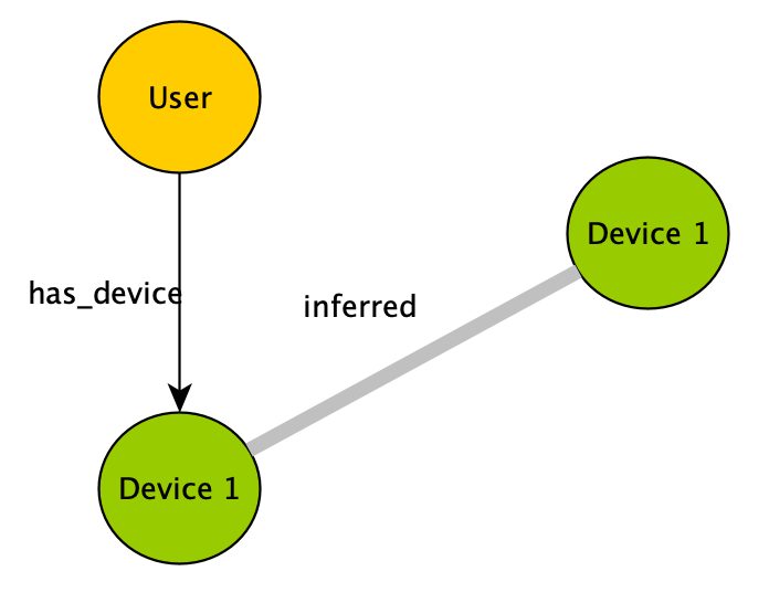
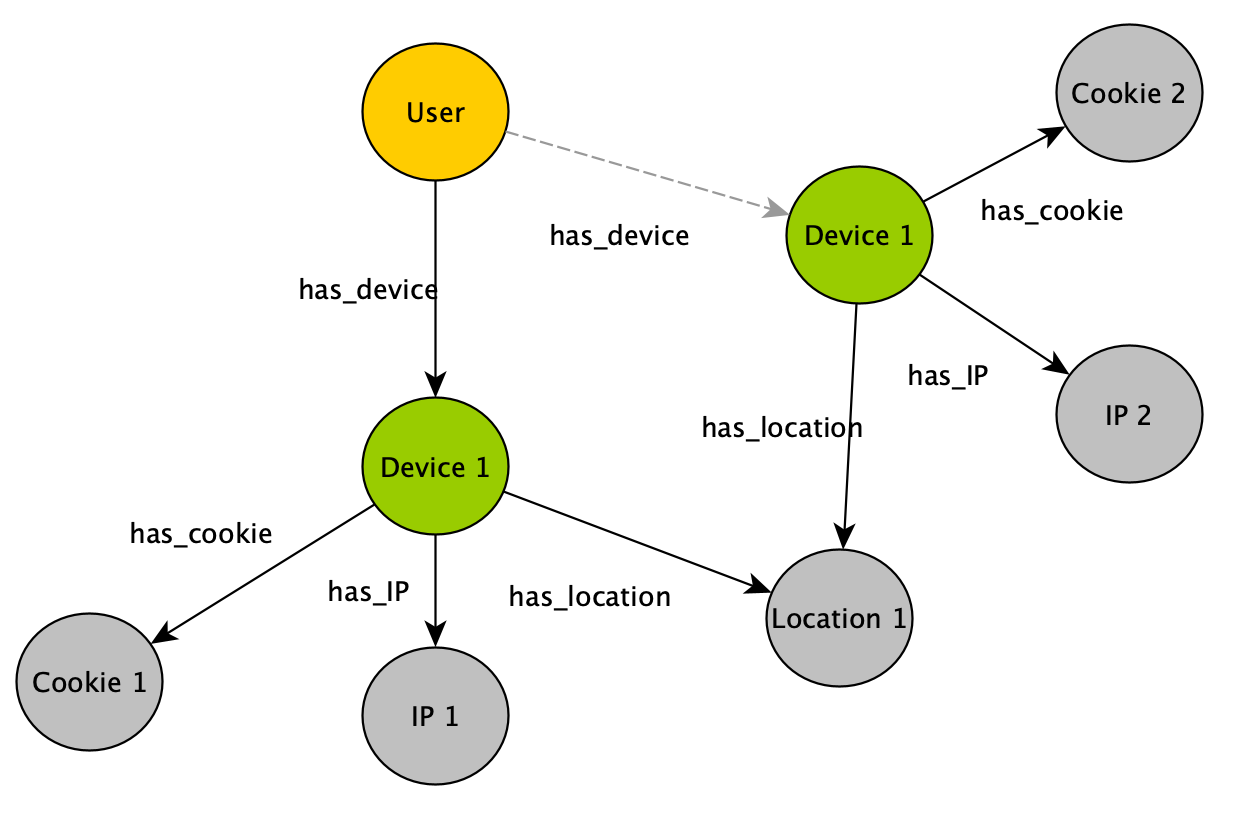
  • link prediction (aka graph completion): predicting new edges. For instance, inferring terroristic affiliations based on social interactions and geolocation.

Drug repurposing is a special type of link prediction: it attempts to find edges between compounds and diseases which have not been considered yet. Looking at our DRKG graph it means that we are interested in edges between the Compound and Disease entity types. It doesn’t mean that other edges are of no importance. Indeed, a generic link prediction pipeline will discover patterns between arbitrary entities and one can focus equally well on new Gene-Gene interactions or symptoms indicating possible diseases.

Note that there is are many names out there to denote the same thing. Geometric (deep) learning, graph embeddings, graph neural networks, graph machine learning, non-Euclidean ML, graph signal processing… all emphasize different aspects of the same research or technology. They all have in common the use of neural networks to learn patterns in graph-like data.

On a technical level, there are heaps of frameworks and techniques with varying quality and sophistication. For drug repositioning specifically you will find the following valuable:

  • Deep Purpose A deep learning library for compound and protein modeling.
  • DRKG The data source also contain various notebooks explaining how to perform various prediction on DRKG.
  • DGL-KE Based on the DGL library, it focuses in learning large scale knowledge graphs and embeddings.
  • TorchDrug A framework designed for drug discovery.

These high-level frameworks hide a lower-level of complexity where you have more grip on assembling neural nets but it also comes with a learning curve. More specifically, PyTorch Geometric, DGL, StellarGraph and TensorFlow Geometric are the most prominent graph machine learning framework.

Crafting and training neural networks is an art and a discipline on its own. It also demands huge processing power if you have any significant dataset. In our case, the DRKG graph with its 5.8 million edges will take you days even with GPU power at your disposal. Still, if you want to train a link prediction model without lots of code, we’ll show it the next section how to proceed. Thereafter we’ll explain how you can make use of pre-trained models to bypass the demanding training phase and get straight to the drup repositioning.

How to train a link prediction model using TorchDrug

As highlighted above, you can craft your own neural net but there are nowadays plenty of high-level frameworks easing the process. TorchDrug is one such framework and it comes with lots of goodies to make one smile. As the name indicates, it’s also geared towards drug discovery, protein representation learning and biomedical graph reasoning in general.

Make sure you have PyTorch installed, as well as Pandas and Numpy. See the ‘Setup’ section below.

TorchDrug has many datasets included by default but not DRKG. It does have Hetionet, which is a subset of DRKG. Creating a dataset is, however, just a dozen lines:

import torch, os
from torch.utils import data as torch_data
from torchdrug import core, datasets, tasks, models, data, utils


class DRKG(data.KnowledgeGraphDataset):
    """
    DRKG for knowledge graph reasoning.

    Parameters:
        path (str): path to store the dataset
        verbose (int, optional): output verbose level
    """

    url = "https://dgl-data.s3-us-west-2.amazonaws.com/dataset/DRKG/drkg.tar.gz"
    md5 = "40519020c906ffa9c821fa53cd294a76"
    def __init__(self, path, verbose = 1):
        path = os.path.expanduser(path)
        if not os.path.exists(path):
            os.makedirs(path)
        self.path = path
        zip_file = utils.download(self.url, path, md5 = self.md5)
        tsv_file = utils.extract(zip_file, "drkg.tsv")
        self.load_tsv(tsv_file, verbose = verbose)

From here on you can use the whole API of TorchDrug and training a link prediction, in particular, is as simple as:

dataset = DRKG("~/data")

lengths = [int(0.8 * len(dataset)), int(0.1 * len(dataset))]
lengths += [len(dataset) - sum(lengths)]
train_set, valid_set, test_set = torch_data.random_split(dataset, lengths)

train_set, valid_set, test_set = torch_data.random_split(dataset, lengths)
print("train: ", len(train_set), "val: ", len(valid_set), "test: ", len(test_set))

model = models.RotatE(num_entity = dataset.num_entity,
                      num_relation = dataset.num_relation,
                      embedding_dim = 2048, max_score = 9)

task = tasks.KnowledgeGraphCompletion(model, num_negative = 256,
                                      adversarial_temperature = 1)

optimizer = torch.optim.Adam(task.parameters(), lr = 2e-5)
solver = core.Engine(task, train_set, valid_set, test_set, optimizer,
                      batch_size = 1024)
solver.train(num_epoch = 200)

First, a an instance of the DRKG dataset is created and it will automatically download the data to the specified directory (here, in the user’s directory ~/data) if not present already. Like any other ML task, a split of the data into training, validation and test happens next. Note that splitting a graph into separate sets is in general a non-trivial task due to edges having to be dropped in order to separate a graph. In this case, the raw data is a simple list of triples and the split is, hence, just an array split.

A semantic triple consists of a subject, a predicate and an object. This corresponds, respectively, to the three parts of an arrow: head, link and tail. In ML context you often will see (h,r,t) rather than the semantic (s,p,o) notation but the two are equivalent.

The rotatE model is an embedding of the graph using relational rotation in complex space as described here. TorchDrug has various embedding algorithms and you can read also more about this in a related article we wrote with Tomaz Bratnic. This embedding step is effectively where the neural net ‘learns’ to recognize patterns in the graph.

The link prediction task KnowledgeGraphCompletion uses the patterns recognized in the model to make predictions. This high-level method hides the tricky parts you need to master if you assemble a net manually.

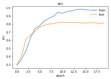
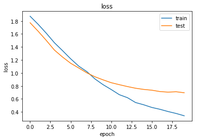
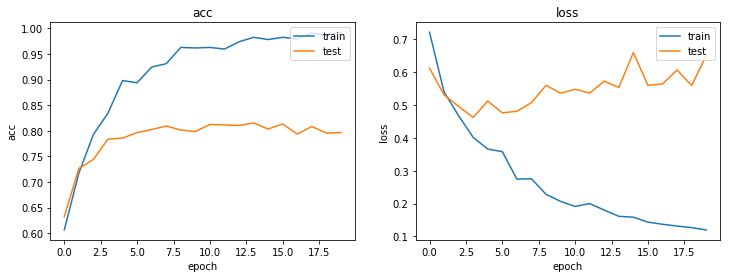
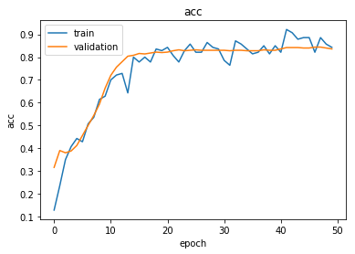
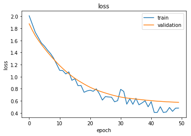
Finally, the net is trained and this does not differ much from any Torch learning loop (or any other deep learning process for that matter). The number of epochs refers to how many times the data is ‘seen’ by the net and a single epoch can take up to an hour with a K80 Nvidia GPU. The large number of edges is of course the culprit here. If you want to fully train the net with an acceptable accuracy (technically, a cross-entropy below 0.2) you will need patience or a special budget. This is the reason that pretrained models are a great shortcut and the situation is similar, for example, with NLP transformers like GPT3 where it often doesn’t make sense to train a model from scratch but rather make stylistic variations of an existing one.

Drug repositioning the easy way

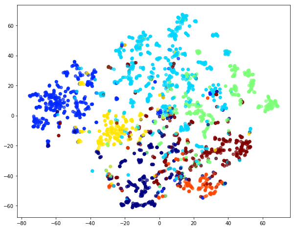
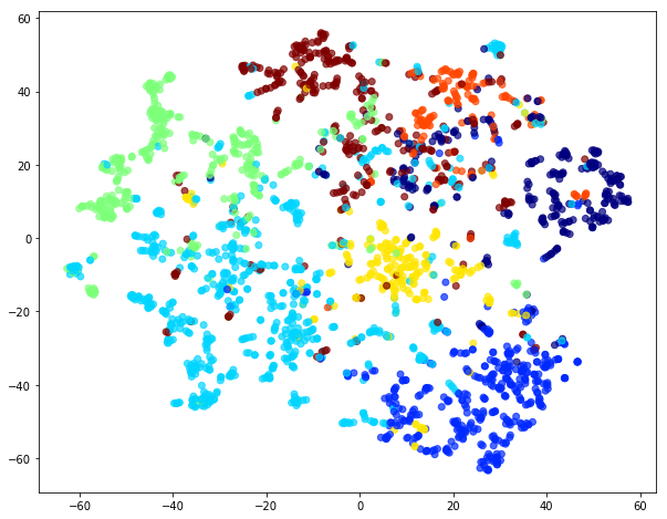
Just like there are various pre-trained models for NLP tasks, you can find embeddings for public datasets like DRKG. A pre-trained model for DRKG consists of vectors for each node and each edge, representing the graph elements in a (high-dimensional) vector space (also know as latent space). These embeddings can exist on their own without the need to deserialize the data back into a model, like the rotatE model above. The (node or edge) vectors effectively capture all there is to know about both the way they sit in the graph (i.e. purely topological information) and their payload (attributes or properties). Typcally, the more two vectors are similar, the more the nodes are similar in a conceptual sense. There are many ways to define ‘similar’ just like there are many ways to define distance in a topological vector space but this is beyond the scope of this article.

To be concrete, we’ll focus on finding new compounds to treat hypertension. In the DRKG graph this corresponds to node with identifier “Disease::DOID:10763”.

The possible edges can have one of the following two labels:

allowed_labels = ['GNBR::T::Compound:Disease','Hetionet::CtD::Compound:Disease']

Furthermore, we will only accept FDA approved compounds to narrow down the options:

allowed_drug = []
with open("./FDAApproved.tsv", newline='', encoding='utf-8') as csvfile:
    reader = csv.DictReader(csvfile, delimiter='\t', fieldnames=['drug','ids'])
    for row_val in reader:
        allowed_drug.append(row_val['drug'])

giving around 2100 possible compounds.

Pretrained models (well, models and graphs in general) don’t work well with concrete names but have numerical identifiers, so one needs a mapping between an actual entity name and a numerical identifier. So, you’ll often find a pretrained model file sitting next to a coupld of dictionaries:

# path to the dictionaries
entity_to_id = './entityToId.tsv'
relation_to_id = './relationToId.tsv'

entity_name_to_id = {}
entity_id_to_name = {}
relation_name_to_id = {}

with open(entity_to_id, newline='', encoding='utf-8') as csvfile:
    reader = csv.DictReader(csvfile, delimiter='\t', fieldnames=['name','id'])
    for row_val in reader:
        entity_name_to_id[row_val['name']] = int(row_val['id'])
        entity_id_to_name[int(row_val['id'])] = row_val['name']

with open(relation_to_id, newline='', encoding='utf-8') as csvfile:
    reader = csv.DictReader(csvfile, delimiter='\t', fieldnames=['name','id'])
    for row_val in reader:
        relation_name_to_id[row_val['name']] = int(row_val['id'])


allowed_drug_ids = []
disease_ids = []
for drug in allowed_drug:
    allowed_drug_ids.append(entity_name_to_id[drug])

for disease in what_diseases:
    disease_ids.append(entity_name_to_id[disease])

allowed_relation_ids = [relation_name_to_id[treat]  for treat in allowed_labels]

Now we are good to load the pretrained vectors:

entity_emb = np.load('./entity_vectors.npy')
rel_emb = np.load('./relation_vectors.npy')

allowed_drug_ids = torch.tensor(allowed_drug_ids).long()
disease_ids = torch.tensor(disease_ids).long()
allowed_relation_ids = torch.tensor(allowed_relation_ids)

allowed_drug_tensors = torch.tensor(entity_emb[allowed_drug_ids])
allowed_relation_tensors = [torch.tensor(rel_emb[rid]) for rid in allowed_relation_ids]

The entity embedding consists of 97238 vectors, matching the amount of nodes in DRKG. Complementary to this, the relation embedding consists of 107 for the 107 types of edges in DRKG. The hypertension node identifer is 83430 corresponding to “Disease::DOID:10763” label.

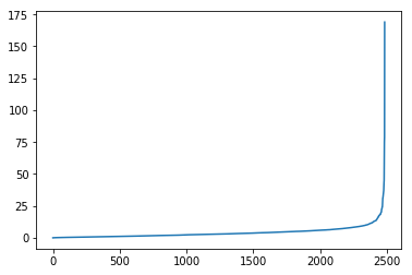
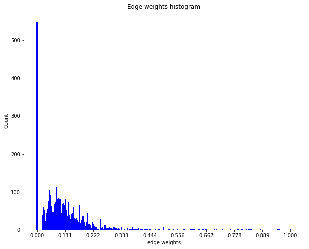
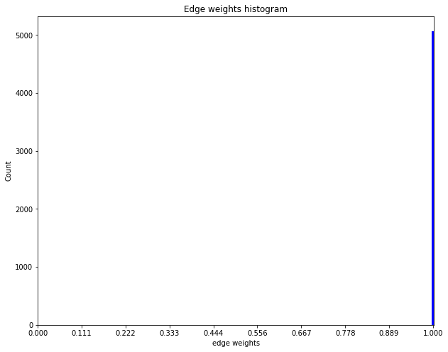
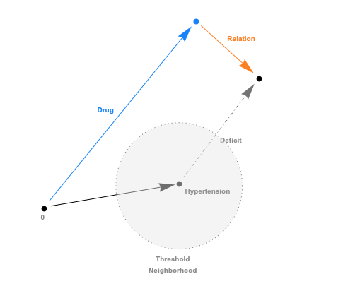
The embeddings can now be used with a standard (Euclidean) metric but to differentiate fitness it’s often more convenient to use a measure which penalizes long distances. It’s a bit like molcular interaction forces (the so-called Lennard-Jones potential)where only the short range matters. This scoring measure (shown In the plot below) quickly diverges beyond a threshold which can be set to accept more or fewer drugs. In the context of differential geometry one would speak of curvature as a measure of deficit between two parallel transports. If the deficit vector is within the threshold neighborhood it’s accepted as a treatment, otherwise the score quickly fades to large values. The fact that the score is negative is simply an easy way to sort the results. The closer the score it to zero the more it’s a perfect fit to treat hypertension.

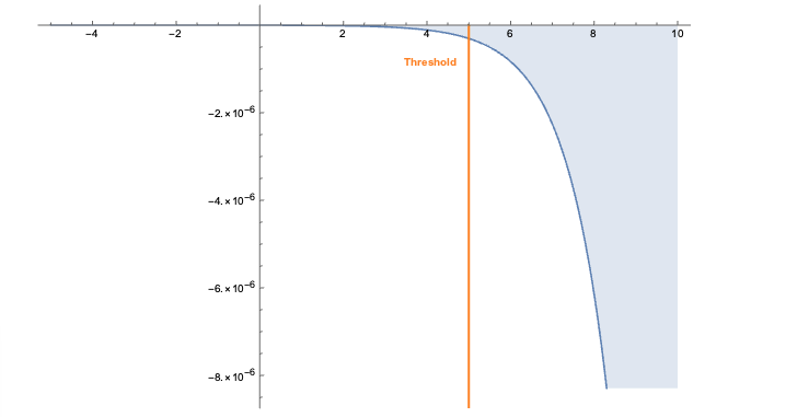
In code this idea is simply this:

threshold= 20
def score(h, r, t):
    return fn.logsigmoid(threshold - torch.norm(h + r - t, p=2, dim=-1))

allowed_drug_scores = []
drug_ids = []
for relation_tensor in range(len(allowed_relation_tensors)):
    rel_vector = allowed_relation_tensors[relation_tensor]
    for disease_id in disease_ids:
        disease_vector = entity_emb[disease_id]
        drug_score = score(allowed_drug_tensors, rel_vector, disease_vector)
        allowed_drug_scores.append(drug_score)
        drug_ids.append(allowed_drug_ids)
scores = torch.cat(allowed_drug_scores)
drug_ids = torch.cat(drug_ids)

Finally, the compound/drugs found are collected and the identifier converted back to actual labels. The result is

Compound::DB00584	-1.883488948806189e-05
Compound::DB00521	-2.2053474822314456e-05
Compound::DB00492	-2.586808113846928e-05
...

and the most likely candidate is Enalapril (DB00584 is the DrugBank Accession Number) which can be checked as a actual drug to treat hypertension.

You should note that with the code above you only have to alter the disease identifier to extract a prediction for that particular disease. Using the Drug Bank you can look up the Accession Number, if necessary.

Another important things to emphasize is the sheer speed with which predictions are made thanks to the pretrained vectors. In effect, you can hook this up via triggers to automatically make prediction when the knowledge graph is changed. Such a setup would be similar to what one designs for fraud detection and, in general, realtime anomaly detection of transactions. Feeding back the link predictions to TigerGraph is really just a REST call away.

Challenges

The small amount of code necessary to achieve all this hides a lot of sophisticated machine learning under the hood. To correctly design and train a graph machine learning pipeline on top of DRKG requires, as mentioned earlier, a lot of time and GPU power. Although the knowledge graph contains plenty of valuable information, it’s all topological. That is, the nodes and edges don’t contain any data and a much more refined drug repurposing model would be possible if e.g. molecular properties, symptom details and other data would be included. This would, however, engender the creation of more complext neural net and more data would mean longer training times (more epochs).

There are also a number of non-technical downsides to drug repositioning:

  • the dosage required for the treatment of a disease usually differs from that of its original target disease, and if this happens, the discovery team will have to begin from Phase I clinical trials. This effectively strips drug repurposing of its advantages over classic drug discovery.
  • no matter how big the knowledge graph is, nothing replaces the expertise and scientific know-how of professionals. Obviously, one shouldn’t narrow down the discovery of treatments and compounds to an algorithm. Graph machine learning is an incentive, not a magic wand.
  • patent right issues can be very complicated for drug repurposing due to the lack of experts in the legal area of drug repositioning, the disclosure of repositioning online or via publications, and the extent of the novelty of the new drug purpose. See the article “Overcoming the legal and regulatory barriers to drug repurposing” for a good overview.

References

Books:

Articles:

TigerGraph:

Data:

  • DRKG The 5.8 million triples a click away.
  • Drug Bank Drug database and more.
  • Clinical Trials ClinicalTrials.gov is a database of privately and publicly funded clinical studies conducted around the world.

Frameworks:

  • Deep Purpose A Deep Learning Library for Compound and Protein Modeling DTI, Drug Property, PPI, DDI, Protein Function Prediction.
  • DGL Easy deep learning on graphs.
  • TorchDrug Easy drug discovery (and much more).
  • StellarGraph Wonderful generic graph machine learning package.
  • PyTorch Geometric Pretty much the de facto deep learning framework.
  • TensorFlow Geometric Similar to PyTorch, but a bit late to the party (ie. more recent and less mature).

Setup

All the files you need are in the Github repo except for the two files containing the pretrained vectors (you can find them here).

Make sure you have Python installed (at least 3.8 and at least 3.9 if you have Apple Silicon) as well as TorchDrug, Numpy and Pandas. Of course, you better have all this in a separate environment.

conda create --name repurpose python=3.9
conda activate repurpose
conda install numpy pandas pyTigerGraph
conda install pytorch -c pytorch
pip install torchdrug
conda install jupyter

Create a free TigerGraph database and for this database create a secret as described above. Check that you can connect to your database with something like this

import pyTigerGraph as tg
host = 'https://your-organization.i.tgcloud.io'
secret = "your-secret"
graph_name = "drkg"
user_name = "tigergraph"
password = "your-password"
token = tg.TigerGraphConnection(host=host, graphname=graph_name, username=user_name, password=password).getToken(secret, "1000000")[0]
conn = tg.TigerGraphConnection(host=host, graphname=graph_name, username=user_name, password=password, apiToken=token)
conn.echo()

You don’t have to download the DRKG data if you use the torchDrugModel.py file since it will download it for you. If you want to download the data to upload to TigerGraph, use this file.

The CreateSchema.ipynb notebook will help you upload the TigerGraph schema and the hypertensionRepositioning.ipnb notebook contains the code described in this article.

We all leave traces of our activity online and use more and more devices for entertainment and professional purposes. Browser cookies, IP address, location info…are routinely recorded and processed by tons of companies trying to figure out who you are, what you do, where you have been and most importantly how to influence your behavior. There are two opposing forces operating in this pool of data. On the one hand, marketing (and similar) companies try to figure out our activity online in order to fine tune ads and other influences. On the other hand, apps and companies help us to hide as much as possible by means of clever tricks and tools (e.g. iCloud Private Relay). It’s a cat and mouse game. In some domains like fraud prevention and anti-terrorism this is not so much a game as a vital activity to keep the world safe.

Entity resolution approach helps companies make inferences across vast volumes of information in enterprise systems and applications by bringing together records that correspond to the same entity.

Although you leave plenty of crumbles behind when visiting sites and places, trying to consolidate all this into something that reflects you as an identity or user is far from easy. For example, if you visit Amazon (without being logged in) on your phone while commuting your location info can’t reliably be used to identify you. Can an IP address be used and how to define distance (a metric) in the space of IP addresses. Nowadays plenty of websites ask a confirmation to see whether you are the same user if they detect anomalies in your location or device used, even if you have the right credentials. Trying to figure out who you are and whether new evidence can be mapped to you is referred to as ‘entity resolution’. The growth of services and diversity in devices has boosted this domain into a major business activity, similar to fraud detection and spam detection. The sophistication in techniques parallels the sophistication of criminal online acivity.

Basic entity resolution doesn’t have to be high-tech however. Some datasets and schemas can be approached with fairly simple techniques. You don’t always have to go straight to graph embeddings and advance graph machine learning. Entity resolution on a graph level corresponds to predicting edges on the basis of harvested user trails. If you want to learn from the payload contained in the nodes you would typically use GraphSAGE or node embedding techniques (using StellarGraph or PyG). A more shallow but faster and often good-enough approach is to use standard graph analytics and learn only from the topological information (i.e. ignore the payload of the nodes and edges).

Let’s take a simple schema where a device is detected together with its IP address and cookies. If the user or identity is known (via login or other) the device used can be linked to the user. If the same user uses another device without login the question is how to link with some confidence (read: probability) this device to the known user. That is, how can the edge between the existing user node and the device node be predicted?

Basic schema

Of course, without any overlap there is no correlation. Depending on the business context you can use whatever makes sense to infer things. Let’s say the location is the same. The ‘same’ is something you need to define in your specific case. Technically it often amounts to defining a metric in the feature space under consideration. The representation below where the location is shared by two devices is created by means of data augmentation. Prior to creating nodes and edges there is some feature engineering cleaning the incoming data, trying to transform it (geolocation of IP address e.g.) and storing it according to the schema. Whether you use a semantic store or a property graph makes a big difference here. Unicity of nodes is automatic in triple stores while this has to be manually enforce in property graphs (specifically, in Neo4j).

Inferred affinity

Inferred identity

The standard approach is to reduce the raw graph by replacing shared information with edges like in the adjacent image. Ones device nodes are linked trough some measure/probability of affinitiy and one of the devices has an identiy, it’s just a matter of cluster things to the known user. The more two devices share nodes, the more likely they are from the same user.

If you transform gradually your raw data to a reduced graph where only identity nodes and device nodes remain the link prediction problem becomes trivial. In some cases you can even shortcut the effort by means of well-known link prediction algorithms like the Jaccard index, Adamic Adar or Soundarajan and Hopcroft.

We have found in multiple cases/projects that the (purely topological) approximation without taking the node payload intoc account is sufficient for most customers. Though in some cases you do need to apply advance machine learning, it comes with a hefty amount of processing and infrastructure.

It should also be noted that if your graph spans millions of nodes there is the marvelous rapids.ai package which easily handles really big graphs. It does not contain graph machine learning but you will find [the aforementioned topological link prediction algorithms](https://docs.rapids.ai/api/cugraph/nightly/api_docs/link_prediction.html).

If you want to discuss your particular entity resolution problem, drop us a line.

Intro

We have shown in related articles how StellarGraph can be used for node and linke predictions using diverse algorithms. All these algorithms effectively turn a graph structure into a more flat (tabular) structure so one can use traditional machine learning algorithms. For example, a random graph walk can collect inforation about the topology of a graph and this data can be added to the existing payload attached to a node or an edge. Using these intermediate ‘tricks’ one can in principle consume any of the existing machine learning approaches and frameworks. Keras and TensorFlow are no exception. You only need to work your way towards appropriate input and output adapter to ingest graph data.
TensorFlow has a separate development branch dedicated to graph learning which they call Neural Structured Learning (NSL). Much like their TensorFlow Probabilty framework for probabilistic reasoning and other TensorFlow extensions it’s a mixed bag; it can allow you to get things done but it also feels unpolished and the API is inpenetrable. On the other hand, if your pipeline is relying on TensorFlow code then this can be a way to increase your models by including graph data (like knowledge graphs or ontologies).
In this article the NSL extension is used to approach our favorite Cora dataset. The takeaway from the explanation is this:

  • in comparison to frameworks like StellarGraph (and other frameworks specifically designed to apply machine learning on graphs) the Keras/TensorFlow code needed to achieve similar results is tremendous. You have a lot of flexibility but it feels more like an uncharted territory than flexibility.
  • the data transformation necessary to make things happen is way more complex as well.
  • if you wish to include graph learning in your (business) projects you are better off with StellarGraph
  • the increased accuracy obtained by including graph data in the ‘normal’ data is not spectacular but can be significant in some domains (say cancer research or predictive analytics).

Setup and imports

    !pip install tf-nightly==2.2.0.dev20200119
    !pip install neural-structured-learning
    from __future__ import absolute_import, division, print_function, unicode_literals
    import neural_structured_learning as nsl
    import tensorflow as tf

The Cora dataset

We have used the dataset over and over again in previous articles and there is a separate article explaining in detail how to download it and how to interprete the data.
In contrast with StellarGraph the Cora set needs to be converted into a TFRecord format:

  1. Generate neighbor features using the original node features and the graph.
  2. Generate train and test data splits containing tf.train.Example instances.
  3. Persist the resulting train and test data in the TFRecord format.

The code necessary to do this is straightforward and convoluted at the same time:

    """Tool that preprocesses Cora data for Graph Keras trainers.
    The Cora dataset can be downloaded from:
    https://linqs-data.soe.ucsc.edu/public/lbc/cora.tgz
    In particular, this tool does the following:
    (a) Converts Cora data (cora.content) into TF Examples,
    (b) Parses the Cora citation graph (cora.cites),
    (c) Merges/combines the TF Examples and the graph, and
    (d) Writes the training and test data in TF Record format.
    The 'cora.content' has the following TSV format:
      publication_id<TAB>word_1<TAB>word_2<TAB>...<TAB>publication_label
    Each line of cora.content is a publication that:
    - Has an integer 'publication_id'
    - Described by a 0/1-valued word vector indicating the absence/presence of the
      corresponding word from the dictionary. In other words, each 'word_k' is
      either 0 or 1.
    - Has a string 'publication_label' representing the publication category.
    The 'cora.cites' is a TSV file that specifies a graph as a set of edges
    representing citation relationships among publications. 'cora.cites' has the
    following TSV format:
      source_publication_id<TAB>target_publication_id
    Each line of cora.cites represents an edge that 'source_publication_id' cites
    'target_publication_id'.
    This tool first converts all the 'cora.content' into TF Examples. Then for
    training data, this tool merges into each labeled Example the features of that
    Example's neighbors according to that instance's edges in the graph. Finally,
    the merged training examples are written to a TF Record file. The test data
    will be written to a TF Record file w/o joining with the neighbors.
    Sample usage:
    $ python preprocess_cora_dataset.py --max_nbrs=5
    """
    from __future__ import absolute_import
    from __future__ import division
    from __future__ import print_function
    import collections
    import random
    import time
    from absl import app
    from absl import flags
    from absl import logging
    from neural_structured_learning.tools import graph_utils
    import six
    import tensorflow as tf
    FLAGS = flags.FLAGS
    FLAGS.showprefixforinfo = False
    flags.DEFINE_string(
        'input_cora_content', '/tmp/cora/cora.content',
        """Input file for Cora content that contains ID, words and labels.""")
    flags.DEFINE_string('input_cora_graph', '/tmp/cora/cora.cites',
                        """Input file for Cora citation graph in TSV format.""")
    flags.DEFINE_integer(
        'max_nbrs', None,
        'The maximum number of neighbors to merge into each labeled Example.')
    flags.DEFINE_float(
        'train_percentage', 0.8,
        """The percentage of examples to be created as training data. The rest
        are created as test data.""")
    flags.DEFINE_string(
        'output_train_data', '/tmp/cora/train_merged_examples.tfr',
        """Output file for training data merged with graph in TF Record format.""")
    flags.DEFINE_string('output_test_data', '/tmp/cora/test_examples.tfr',
                        """Output file for test data in TF Record format.""")
    def _int64_feature(*value):
      """Returns int64 tf.train.Feature from a bool / enum / int / uint."""
      return tf.train.Feature(int64_list=tf.train.Int64List(value=list(value)))
    def parse_cora_content(in_file, train_percentage):
      """Converts the Cora content (in TSV) to `tf.train.Example` instances.
      This function parses Cora content (in TSV), converts string labels to integer
      label IDs, randomly splits the data into training and test sets, and returns
      the training and test sets as outputs.
      Args:
        in_file: A string indicating the input file path.
        train_percentage: A float indicating the percentage of training examples
          over the dataset.
      Returns:
        train_examples: A dict with keys being example IDs (string) and values being
        `tf.train.Example` instances.
        test_examples: A dict with keys being example IDs (string) and values being
        `tf.train.Example` instances.
      """
      # Provides a mapping from string labels to integer indices.
      label_index = {
          'Case_Based': 0,
          'Genetic_Algorithms': 1,
          'Neural_Networks': 2,
          'Probabilistic_Methods': 3,
          'Reinforcement_Learning': 4,
          'Rule_Learning': 5,
          'Theory': 6,
      }
      # Fixes the random seed so the train/test split can be reproduced.
      random.seed(1)
      train_examples = {}
      test_examples = {}
      with open(in_file, 'rU') as cora_content:
        for line in cora_content:
          entries = line.rstrip('\n').split('\t')
          # entries contains [ID, Word1, Word2, ..., Label]; 'Words' are 0/1 values.
          words = map(int, entries[1:-1])
          features = {
              'words': _int64_feature(*words),
              'label': _int64_feature(label_index[entries[-1]]),
          }
          example_features = tf.train.Example(
              features=tf.train.Features(feature=features))
          example_id = entries[0]
          if random.uniform(0, 1) <= train_percentage:  # for train/test split.
            train_examples[example_id] = example_features
          else:
            test_examples[example_id] = example_features
      return train_examples, test_examples
    def _join_examples(seed_exs, nbr_exs, graph, max_nbrs):
      r"""Joins the `seeds` and `nbrs` Examples using the edges in `graph`.
      This generator joins and augments each labeled Example in `seed_exs` with the
      features of at most `max_nbrs` of the seed's neighbors according to the given
      `graph`, and yields each merged result.
      Args:
        seed_exs: A `dict` mapping node IDs to labeled Examples.
        nbr_exs: A `dict` mapping node IDs to unlabeled Examples.
        graph: A `dict`: source -> (target, weight).
        max_nbrs: The maximum number of neighbors to merge into each seed Example,
          or `None` if the number of neighbors per node is unlimited.
      Yields:
        The result of merging each seed Example with the features of its neighbors,
        as described by the module comment.
      """
      # A histogram of the out-degrees of all seed Examples. The keys of this dict
      # range from 0 to 'max_nbrs' (inclusive) if 'max_nbrs' is finite.
      out_degree_count = collections.Counter()
      def has_ex(node_id):
        """Returns true iff 'node_id' is in the 'seed_exs' or 'nbr_exs dict'."""
        result = (node_id in seed_exs) or (node_id in nbr_exs)
        if not result:
          logging.warning('No tf.train.Example found for edge target ID: "%s"',
                          node_id)
        return result
      def lookup_ex(node_id):
        """Returns the Example from `seed_exs` or `nbr_exs` with the given ID."""
        return seed_exs[node_id] if node_id in seed_exs else nbr_exs[node_id]
      def join_seed_to_nbrs(seed_id):
        """Joins the seed with ID `seed_id` to its out-edge graph neighbors.
        This also has the side-effect of maintaining the `out_degree_count`.
        Args:
          seed_id: The ID of the seed Example to start from.
        Returns:
          A list of (nbr_wt, nbr_id) pairs (in decreasing weight order) of the
          seed Example's top `max_nbrs` neighbors. So the resulting list will have
          size at most `max_nbrs`, but it may be less (or even empty if the seed
          Example has no out-edges).
        """
        nbr_dict = graph[seed_id] if seed_id in graph else {}
        nbr_wt_ex_list = [(nbr_wt, nbr_id)
                          for (nbr_id, nbr_wt) in six.iteritems(nbr_dict)
                          if has_ex(nbr_id)]
        result = sorted(nbr_wt_ex_list, reverse=True)[:max_nbrs]
        out_degree_count[len(result)] += 1
        return result
      def merge_examples(seed_ex, nbr_wt_ex_list):
        """Merges neighbor Examples into the given seed Example `seed_ex`.
        Args:
          seed_ex: A labeled Example.
          nbr_wt_ex_list: A list of (nbr_wt, nbr_id) pairs (in decreasing nbr_wt
            order) representing the neighbors of 'seed_ex'.
        Returns:
          The Example that results from merging the features of the neighbor
          Examples (as well as creating a feature for each neighbor's edge weight)
          into `seed_ex`. See the `join()` description above for how the neighbor
          features are named in the result.
        """
        # Make a deep copy of the seed Example to augment.
        merged_ex = tf.train.Example()
        merged_ex.CopyFrom(seed_ex)
        # Add a feature for the number of neighbors.
        merged_ex.features.feature['NL_num_nbrs'].int64_list.value.append(
            len(nbr_wt_ex_list))
        # Enumerate the neighbors, and merge in the features of each.
        for index, (nbr_wt, nbr_id) in enumerate(nbr_wt_ex_list):
          prefix = 'NL_nbr_{}_'.format(index)
          # Add the edge weight value as a new singleton float feature.
          weight_feature = prefix + 'weight'
          merged_ex.features.feature[weight_feature].float_list.value.append(nbr_wt)
          # Copy each of the neighbor Examples features, prefixed with 'prefix'.
          nbr_ex = lookup_ex(nbr_id)
          for (feature_name, feature_val) in six.iteritems(nbr_ex.features.feature):
            new_feature = merged_ex.features.feature[prefix + feature_name]
            new_feature.CopyFrom(feature_val)
        return merged_ex
      start_time = time.time()
      logging.info(
          'Joining seed and neighbor tf.train.Examples with graph edges...')
      for (seed_id, seed_ex) in six.iteritems(seed_exs):
        yield merge_examples(seed_ex, join_seed_to_nbrs(seed_id))
      logging.info(
          'Done creating and writing %d merged tf.train.Examples (%.2f seconds).',
          len(seed_exs), (time.time() - start_time))
      logging.info('Out-degree histogram: %s', sorted(out_degree_count.items()))
    def main(unused_argv):
      start_time = time.time()
      # Parses Cora content into TF Examples.
      train_examples, test_examples = parse_cora_content(FLAGS.input_cora_content,
                                                         FLAGS.train_percentage)
      graph = graph_utils.read_tsv_graph(FLAGS.input_cora_graph)
      graph_utils.add_undirected_edges(graph)
      # Joins 'train_examples' with 'graph'. 'test_examples' are used as *unlabeled*
      # neighbors for transductive learning purpose. In other words, the labels of
      # test_examples are not used.
      with tf.io.TFRecordWriter(FLAGS.output_train_data) as writer:
        for merged_example in _join_examples(train_examples, test_examples, graph,
                                             FLAGS.max_nbrs):
          writer.write(merged_example.SerializeToString())
      logging.info('Output training data written to TFRecord file: %s.',
                   FLAGS.output_train_data)
      # Writes 'test_examples' out w/o joining with the graph since graph
      # regularization is used only during training, not testing/serving.
      with tf.io.TFRecordWriter(FLAGS.output_test_data) as writer:
        for example in six.itervalues(test_examples):
          writer.write(example.SerializeToString())
      logging.info('Output test data written to TFRecord file: %s.',
                   FLAGS.output_test_data)
      logging.info('Total running time: %.2f minutes.',
                   (time.time() - start_time) / 60.0)
    if __name__ == '__main__':
      # Ensures TF 2.0 behavior even if TF 1.X is installed.
      tf.compat.v1.enable_v2_behavior()
      app.run(main)

With all of this in place you can run the script on the Cora data like so:

    !python preprocess_cora_dataset.py \
    --input_cora_content=/tmp/cora/cora.content \
    --input_cora_graph=/tmp/cora/cora.cites \
    --max_nbrs=5 \
    --output_train_data=/tmp/cora/train_merged_examples.tfr \
    --output_test_data=/tmp/cora/test_examples.tfr
preprocess_cora_dat 100%[===================>]  11.15K  --.-KB/s    in 0s
2020-02-02 08:25:58 (152 MB/s) - ‘preprocess_cora_dataset.py.1’ saved [11419/11419]
Reading graph file: /tmp/cora/cora.cites...
Done reading 5429 edges from: /tmp/cora/cora.cites (0.01 seconds).
Making all edges bi-directional...
Done (0.00 seconds). Total graph nodes: 2708
Joining seed and neighbor tf.train.Examples with graph edges...
Done creating and writing 2155 merged tf.train.Examples (1.09 seconds).
Out-degree histogram: [(1, 386), (2, 468), (3, 452), (4, 309), (5, 540)]
Output training data written to TFRecord file: /tmp/cora/train_merged_examples.tfr.
Output test data written to TFRecord file: /tmp/cora/test_examples.tfr.
Total running time: 0.04 minutes.

Variables and Hyperparameters

The file paths to the train and test data are based on the command line flag
values used to invoke the ‘preprocess_cora_dataset.py’ script above.

    ### Experiment dataset
    TRAIN_DATA_PATH = '/tmp/cora/train_merged_examples.tfr'
    TEST_DATA_PATH = '/tmp/cora/test_examples.tfr'
    ### Constants used to identify neighbor features in the input.
    NBR_FEATURE_PREFIX = 'NL_nbr_'
    NBR_WEIGHT_SUFFIX = '_weight'

Next, we’ll use a class defining the hyperparameters and constants used for training and evaluation.:

  • dropout_rate: Controls the rate of dropout following each fully
    connected layer
  • num_fc_units: The number of fully connected layers in our neural
    network.
  • train_epochs: The number of training epochs.
  • batch_size: Batch size used for training and evaluation.
  • num_classes: There are a total 7 different classes
  • max_seq_length: This is the size of the vocabulary and all instances in
    the input have a dense multi-hot, bag-of-words representation. In other
    words, a value of 1 for a word indicates that the word is present in the
    input and a value of 0 indicates that it is not.
  • distance_type: This is the distance metric used to regularize the sample
    with its neighbors.
  • graph_regularization_multiplier: This controls the relative weight of
    the graph regularization term in the overall loss function.
  • num_neighbors: The number of neighbors used for graph regularization.
    This value has to be less than or equal to the max_nbrs command-line
    argument used above when running preprocess_cora_dataset.py.
  • eval_steps: The number of batches to process before deeming evaluation
    is complete. If set to None, all instances in the test set are evaluated.

    class HParams(object):
      """Hyperparameters used for training."""
      def __init__(self):
        ### training parameters
        self.train_epochs = 100
        self.batch_size = 128
        self.dropout_rate = 0.5
        ### eval parameters
        self.eval_steps = None  # All instances in the test set are evaluated.
        ### dataset parameters
        self.num_classes = 7
        self.max_seq_length = 1433
        ### neural graph learning parameters
        self.distance_type = nsl.configs.DistanceType.L2
        self.graph_regularization_multiplier = 0.1
        self.num_neighbors = 1
        ### model architecture
        self.num_fc_units = [50, 50]
    HPARAMS = HParams()
    

Train and test data

The preprocessing already transformed the data into train an test data. Now we only have to read it in a mold it into a TFRecordDataset set.

    def parse_example(example_proto):
      """Extracts relevant fields from the `example_proto`.
      Args:
        example_proto: An instance of `tf.train.Example`.
      Returns:
        A pair whose first value is a dictionary containing relevant features
        and whose second value contains the ground truth labels.
      """
      # The 'words' feature is a multi-hot, bag-of-words representation of the
      # original raw text. A default value is required for examples that don't
      # have the feature.
      feature_spec = {
          'words':
              tf.io.FixedLenFeature([HPARAMS.max_seq_length],
                                    tf.int64,
                                    default_value=tf.constant(
                                        0,
                                        dtype=tf.int64,
                                        shape=[HPARAMS.max_seq_length])),
          'label':
              tf.io.FixedLenFeature((), tf.int64, default_value=-1),
      }
      # We also extract corresponding neighbor features in a similar manner to
      # the features above.
      for i in range(HPARAMS.num_neighbors):
        nbr_feature_key = '{}{}_{}'.format(NBR_FEATURE_PREFIX, i, 'words')
        nbr_weight_key = '{}{}{}'.format(NBR_FEATURE_PREFIX, i, NBR_WEIGHT_SUFFIX)
        feature_spec[nbr_feature_key] = tf.io.FixedLenFeature(
            [HPARAMS.max_seq_length],
            tf.int64,
            default_value=tf.constant(
                0, dtype=tf.int64, shape=[HPARAMS.max_seq_length]))
        # We assign a default value of 0.0 for the neighbor weight so that
        # graph regularization is done on samples based on their exact number
        # of neighbors. In other words, non-existent neighbors are discounted.
        feature_spec[nbr_weight_key] = tf.io.FixedLenFeature(
            [1], tf.float32, default_value=tf.constant([0.0]))
      features = tf.io.parse_single_example(example_proto, feature_spec)
      labels = features.pop('label')
      return features, labels
    def make_dataset(file_path, training=False):
      """Creates a `tf.data.TFRecordDataset`.
      Args:
        file_path: Name of the file in the `.tfrecord` format containing
          `tf.train.Example` objects.
        training: Boolean indicating if we are in training mode.
      Returns:
        An instance of `tf.data.TFRecordDataset` containing the `tf.train.Example`
        objects.
      """
      dataset = tf.data.TFRecordDataset([file_path])
      if training:
        dataset = dataset.shuffle(10000)
      dataset = dataset.map(parse_example)
      dataset = dataset.batch(HPARAMS.batch_size)
      return dataset
    train_dataset = make_dataset(TRAIN_DATA_PATH, training=True)
    test_dataset = make_dataset(TEST_DATA_PATH)

To get an idea of how the tensors look like:

    for feature_batch, label_batch in train_dataset.take(1):
      print('Feature list:', list(feature_batch.keys()))
      print('Batch of inputs:', feature_batch['words'])
      nbr_feature_key = '{}{}_{}'.format(NBR_FEATURE_PREFIX, 0, 'words')
      nbr_weight_key = '{}{}{}'.format(NBR_FEATURE_PREFIX, 0, NBR_WEIGHT_SUFFIX)
      print('Batch of neighbor inputs:', feature_batch[nbr_feature_key])
      print('Batch of neighbor weights:',
            tf.reshape(feature_batch[nbr_weight_key], [-1]))
      print('Batch of labels:', label_batch)
Feature list: ['NL_nbr_0_weight', 'NL_nbr_0_words', 'words']
Batch of inputs: tf.Tensor(
[[0 0 0 ... 0 0 0]
 [0 0 0 ... 0 0 0]
 [0 0 0 ... 0 0 0]
 ...
 [0 0 0 ... 0 0 0]
 [0 0 0 ... 0 0 0]
 [0 0 0 ... 0 0 0]], shape=(128, 1433), dtype=int64)
Batch of neighbor inputs: tf.Tensor(
[[0 0 0 ... 0 0 0]
 [0 0 0 ... 0 0 0]
 [0 0 0 ... 0 0 0]
 ...
 [0 0 0 ... 0 0 0]
 [0 0 0 ... 0 0 0]
 [0 0 0 ... 0 0 0]], shape=(128, 1433), dtype=int64)
Batch of neighbor weights: tf.Tensor(
[1. 1. 1. 1. 1. 1. 1. 1. 1. 1. 1. 1. 1. 1. 1. 1. 1. 1. 1. 1. 1. 1. 1. 1.
 1. 1. 1. 1. 1. 1. 1. 1. 1. 1. 1. 1. 1. 1. 1. 1. 1. 1. 1. 1. 1. 1. 1. 1.
 1. 1. 1. 1. 1. 1. 1. 1. 1. 1. 1. 1. 1. 1. 1. 1. 1. 1. 1. 1. 1. 1. 1. 1.
 1. 1. 1. 1. 1. 1. 1. 1. 1. 1. 1. 1. 1. 1. 1. 1. 1. 1. 1. 1. 1. 1. 1. 1.
 1. 1. 1. 1. 1. 1. 1. 1. 1. 1. 1. 1. 1. 1. 1. 1. 1. 1. 1. 1. 1. 1. 1. 1.
 1. 1. 1. 1. 1. 1. 1. 1.], shape=(128,), dtype=float32)
Batch of labels: tf.Tensor(
[1 2 3 1 4 0 4 6 5 2 2 2 4 2 2 4 3 2 3 0 5 6 1 2 2 2 2 0 3 6 6 1 2 1 0 2 2
 4 6 3 6 2 1 2 6 2 5 2 6 1 3 1 0 2 4 1 5 2 2 6 0 2 2 6 5 1 2 0 2 2 6 5 2 2
 2 1 4 1 1 1 2 4 2 2 2 1 3 2 1 6 3 5 0 2 3 2 2 6 4 2 2 4 1 5 4 6 1 3 2 6 0
 3 1 2 2 2 3 2 1 2 4 2 5 0 0 5 6 1], shape=(128,), dtype=int64)

and similarly

    for feature_batch, label_batch in test_dataset.take(1):
      print('Feature list:', list(feature_batch.keys()))
      print('Batch of inputs:', feature_batch['words'])
      nbr_feature_key = '{}{}_{}'.format(NBR_FEATURE_PREFIX, 0, 'words')
      nbr_weight_key = '{}{}{}'.format(NBR_FEATURE_PREFIX, 0, NBR_WEIGHT_SUFFIX)
      print('Batch of neighbor inputs:', feature_batch[nbr_feature_key])
      print('Batch of neighbor weights:',
            tf.reshape(feature_batch[nbr_weight_key], [-1]))
      print('Batch of labels:', label_batch)
Feature list: ['NL_nbr_0_weight', 'NL_nbr_0_words', 'words']
Batch of inputs: tf.Tensor(
[[0 0 0 ... 0 0 0]
 [0 0 0 ... 0 0 0]
 [0 0 0 ... 0 0 0]
 ...
 [0 0 0 ... 0 0 0]
 [0 0 0 ... 0 0 0]
 [0 0 0 ... 0 0 0]], shape=(128, 1433), dtype=int64)
Batch of neighbor inputs: tf.Tensor(
[[0 0 0 ... 0 0 0]
 [0 0 0 ... 0 0 0]
 [0 0 0 ... 0 0 0]
 ...
 [0 0 0 ... 0 0 0]
 [0 0 0 ... 0 0 0]
 [0 0 0 ... 0 0 0]], shape=(128, 1433), dtype=int64)
Batch of neighbor weights: tf.Tensor(
[0. 0. 0. 0. 0. 0. 0. 0. 0. 0. 0. 0. 0. 0. 0. 0. 0. 0. 0. 0. 0. 0. 0. 0.
 0. 0. 0. 0. 0. 0. 0. 0. 0. 0. 0. 0. 0. 0. 0. 0. 0. 0. 0. 0. 0. 0. 0. 0.
 0. 0. 0. 0. 0. 0. 0. 0. 0. 0. 0. 0. 0. 0. 0. 0. 0. 0. 0. 0. 0. 0. 0. 0.
 0. 0. 0. 0. 0. 0. 0. 0. 0. 0. 0. 0. 0. 0. 0. 0. 0. 0. 0. 0. 0. 0. 0. 0.
 0. 0. 0. 0. 0. 0. 0. 0. 0. 0. 0. 0. 0. 0. 0. 0. 0. 0. 0. 0. 0. 0. 0. 0.
 0. 0. 0. 0. 0. 0. 0. 0.], shape=(128,), dtype=float32)
Batch of labels: tf.Tensor(
[5 2 2 2 1 2 6 3 2 3 6 1 3 6 4 4 2 3 3 0 2 0 5 2 1 0 6 3 6 4 2 2 3 0 4 2 2
 2 2 3 2 2 2 0 2 2 2 2 4 2 3 4 0 2 6 2 1 4 2 0 0 1 4 2 6 0 5 2 2 3 2 5 2 5
 2 3 2 2 2 2 2 6 6 3 2 4 2 6 3 2 2 6 2 4 2 2 1 3 4 6 0 0 2 4 2 1 3 6 6 2 6
 6 6 1 4 6 4 3 6 6 0 0 2 6 2 4 0 0], shape=(128,), dtype=int64)

The model

In order to show the difference between normal learning and graph learning we’ll use a base model and a graph’d model.
The sequential base model is a standard MLP with the amount of layers specified in the constant above:

    def make_mlp_sequential_model(hparams):
      """Creates a sequential multi-layer perceptron model."""
      model = tf.keras.Sequential()
      model.add(
          tf.keras.layers.InputLayer(
              input_shape=(hparams.max_seq_length,), name='words'))
      # Input is already one-hot encoded in the integer format. We cast it to
      # floating point format here.
      model.add(
          tf.keras.layers.Lambda(lambda x: tf.keras.backend.cast(x, tf.float32)))
      for num_units in hparams.num_fc_units:
        model.add(tf.keras.layers.Dense(num_units, activation='relu'))
        # For sequential models, by default, Keras ensures that the 'dropout' layer
        # is invoked only during training.
        model.add(tf.keras.layers.Dropout(hparams.dropout_rate))
      model.add(tf.keras.layers.Dense(hparams.num_classes, activation='softmax'))
      return model

The functional base model looks like this

    def make_mlp_functional_model(hparams):
      """Creates a functional API-based multi-layer perceptron model."""
      inputs = tf.keras.Input(
          shape=(hparams.max_seq_length,), dtype='int64', name='words')
      # Input is already one-hot encoded in the integer format. We cast it to
      # floating point format here.
      cur_layer = tf.keras.layers.Lambda(
          lambda x: tf.keras.backend.cast(x, tf.float32))(
              inputs)
      for num_units in hparams.num_fc_units:
        cur_layer = tf.keras.layers.Dense(num_units, activation='relu')(cur_layer)
        # For functional models, by default, Keras ensures that the 'dropout' layer
        # is invoked only during training.
        cur_layer = tf.keras.layers.Dropout(hparams.dropout_rate)(cur_layer)
      outputs = tf.keras.layers.Dense(
          hparams.num_classes, activation='softmax')(
              cur_layer)
      model = tf.keras.Model(inputs, outputs=outputs)
      return model

Finally, we subclass the the MLP model

    def make_mlp_subclass_model(hparams):
      """Creates a multi-layer perceptron subclass model in Keras."""
      class MLP(tf.keras.Model):
        """Subclass model defining a multi-layer perceptron."""
        def __init__(self):
          super(MLP, self).__init__()
          # Input is already one-hot encoded in the integer format. We create a
          # layer to cast it to floating point format here.
          self.cast_to_float_layer = tf.keras.layers.Lambda(
              lambda x: tf.keras.backend.cast(x, tf.float32))
          self.dense_layers = [
              tf.keras.layers.Dense(num_units, activation='relu')
              for num_units in hparams.num_fc_units
          ]
          self.dropout_layer = tf.keras.layers.Dropout(hparams.dropout_rate)
          self.output_layer = tf.keras.layers.Dense(
              hparams.num_classes, activation='softmax')
        def call(self, inputs, training=False):
          cur_layer = self.cast_to_float_layer(inputs['words'])
          for dense_layer in self.dense_layers:
            cur_layer = dense_layer(cur_layer)
            cur_layer = self.dropout_layer(cur_layer, training=training)
          outputs = self.output_layer(cur_layer)
          return outputs
      return MLP()

Using of the above we can output the characteristics of our base model

    base_model_tag, base_model = 'FUNCTIONAL', make_mlp_functional_model(HPARAMS)
    base_model.summary()
Model: "model"
_________________________________________________________________
Layer (type)                 Output Shape              Param #
=================================================================
words (InputLayer)           [(None, 1433)]            0
_________________________________________________________________
lambda (Lambda)              (None, 1433)              0
_________________________________________________________________
dense (Dense)                (None, 50)                71700
_________________________________________________________________
dropout (Dropout)            (None, 50)                0
_________________________________________________________________
dense_1 (Dense)              (None, 50)                2550
_________________________________________________________________
dropout_1 (Dropout)          (None, 50)                0
_________________________________________________________________
dense_2 (Dense)              (None, 7)                 357
=================================================================
Total params: 74,607
Trainable params: 74,607
Non-trainable params: 0
_________________________________________________________________

Training

From here on all is similar to any other learning based on TensorFlow and training our base model is simply:

    base_model.compile(
        optimizer='adam',
        loss='sparse_categorical_crossentropy',
        metrics=['accuracy'])
    base_model.fit(train_dataset, epochs=HPARAMS.train_epochs, verbose=1)
Epoch 1/100
17/17 [==============================] - 0s 26ms/step - loss: 1.9442 - accuracy: 0.1675
Epoch 2/100
17/17 [==============================] - 0s 10ms/step - loss: 1.8739 - accuracy: 0.2770
Epoch 3/100
17/17 [==============================] - 0s 10ms/step - loss: 1.7915 - accuracy: 0.3374
Epoch 4/100
17/17 [==============================] - 0s 13ms/step - loss: 1.6789 - accuracy: 0.3698
...
Epoch 99/100
17/17 [==============================] - 0s 11ms/step - loss: 0.0542 - accuracy: 0.9842
Epoch 100/100
17/17 [==============================] - 0s 11ms/step - loss: 0.0405 - accuracy: 0.9898

Base model accuracy

Our base model achieves a 78% accuracy. Not spectacular but it only serves as a baseline for the next step.

    def print_metrics(model_desc, eval_metrics):
      """Prints evaluation metrics.
      Args:
        model_desc: A description of the model.
        eval_metrics: A dictionary mapping metric names to corresponding values. It
          must contain the loss and accuracy metrics.
      """
      print('\n')
      print('Eval accuracy for ', model_desc, ': ', eval_metrics['accuracy'])
      print('Eval loss for ', model_desc, ': ', eval_metrics['loss'])
      if 'graph_loss' in eval_metrics:
        print('Eval graph loss for ', model_desc, ': ', eval_metrics['graph_loss'])
    eval_results = dict(
        zip(base_model.metrics_names,
            base_model.evaluate(test_dataset, steps=HPARAMS.eval_steps)))
    print_metrics('Base MLP model', eval_results)
      5/Unknown - 0s 22ms/step - loss: 1.2329 - accuracy: 0.7830
Eval accuracy for  Base MLP model :  0.7830018
Eval loss for  Base MLP model :  1.2328713834285736

Graph regularization

Incorporating graph regularization into the loss term of an existing tf.Keras.Model requires just a few lines of code. The base model is wrapped to create a new tf.Keras subclass model, whose loss includes graph regularization.

    base_reg_model_tag, base_reg_model = 'FUNCTIONAL', make_mlp_functional_model(
        HPARAMS)
    # Wrap the base MLP model with graph regularization.
    graph_reg_config = nsl.configs.make_graph_reg_config(
        max_neighbors=HPARAMS.num_neighbors,
        multiplier=HPARAMS.graph_regularization_multiplier,
        distance_type=HPARAMS.distance_type,
        sum_over_axis=-1)
    graph_reg_model = nsl.keras.GraphRegularization(base_reg_model,
                                                    graph_reg_config)
    graph_reg_model.compile(
        optimizer='adam',
        loss='sparse_categorical_crossentropy',
        metrics=['accuracy'])
    graph_reg_model.fit(train_dataset, epochs=HPARAMS.train_epochs, verbose=1)
Epoch 1/100
  "Converting sparse IndexedSlices to a dense Tensor of unknown shape. "
17/17 [==============================] - 1s 78ms/step - loss: 1.9388 - accuracy: 0.1791 - graph_loss: 0.0083
Epoch 2/100
17/17 [==============================] - 0s 12ms/step - loss: 1.8447 - accuracy: 0.3030 - graph_loss: 0.0106
Epoch 3/100
17/17 [==============================] - 0s 13ms/step - loss: 1.7526 - accuracy: 0.3346 - graph_loss: 0.0228
Epoch 4/100
17/17 [==============================] - 0s 11ms/step - loss: 1.6512 - accuracy: 0.3675 - graph_loss: 0.0456
...
Epoch 99/100
17/17 [==============================] - 0s 15ms/step - loss: 0.0825 - accuracy: 0.9870 - graph_loss: 0.3407
Epoch 100/100
17/17 [==============================] - 0s 14ms/step - loss: 0.0823 - accuracy: 0.9856 - graph_loss: 0.3328

Graph regularization accuracy

With graph information added we increase our accuracy to 81% compared to the 78% baseline from above. Again, nothing hyperbolic but it shows that graph regularization leads to an improved model.

    eval_results = dict(
        zip(graph_reg_model.metrics_names,
            graph_reg_model.evaluate(test_dataset, steps= HPARAMS.eval_steps)))
    print_metrics('MLP + graph regularization', eval_results)
      5/Unknown - 0s 68ms/step - loss: 1.0859 - accuracy: 0.8156 - graph_loss: 0.0000e+00
Eval accuracy for  MLP + graph regularization :  0.8155515
Eval loss for  MLP + graph regularization :  1.0859381407499313
Eval graph loss for  MLP + graph regularization :  0.0

In a previous article we explained how GraphSage can be used for link predictions. This article shows that the same method can be used to make predictions on a node level.
The research paper is the same as for link predictions, that is “Inductive Representation Learning on Large Graphs”. Also, like pretty much all graph learning articles on this site, we’ll use the Cora dataset.
Purpose of this article is to show that the ‘subject’ of each paper in the Cora graph can be predicted on the basis of the graph structure together with whatever features are additionally available on the nodes.

    import networkx as nx
    import pandas as pd
    import os
    import stellargraph as sg
    from stellargraph.mapper import GraphSAGENodeGenerator
    from stellargraph.layer import GraphSAGE
    # note that using "from keras" will not work
    from tensorflow.keras import layers, optimizers, losses, metrics, Model
    from sklearn import preprocessing, feature_extraction, model_selection

Data import

Please read through our Cora dataset article to understand a bit what the following code does:

    data_dir = os.path.expanduser("~/data/cora")
    cora_location = os.path.expanduser(os.path.join(data_dir, "cora.cites"))
    g_nx = nx.read_edgelist(path=cora_location)
    cora_data_location = os.path.expanduser(os.path.join(data_dir, "cora.content"))
    node_attr = pd.read_csv(cora_data_location, sep='\t', header=None)
    values = { str(row.tolist()[0]): row.tolist()[-1] for _, row in node_attr.iterrows()}
    nx.set_node_attributes(g_nx, values, 'subject')
    g_nx_ccs = (g_nx.subgraph(c).copy() for c in nx.connected_components(g_nx))
    g_nx = max(g_nx_ccs, key=len)
    feature_names = ["w_{}".format(ii) for ii in range(1433)]
    column_names =  feature_names + ["subject"]
    node_data = pd.read_csv(os.path.join(data_dir, "cora.content"), header=None, names=column_names, sep='\t')
    node_data.index = node_data.index.map(str)
    node_data = node_data[node_data.index.isin(list(g_nx.nodes()))]

The ‘subject’ label on the nodes is what we’ll learn and predict:

    set(node_data["subject"])
{'Case_Based',
 'Genetic_Algorithms',
 'Neural_Networks',
 'Probabilistic_Methods',
 'Reinforcement_Learning',
 'Rule_Learning',
 'Theory'}

Splitting the data

The GraphSage generator takes the graph structure and the node-data as input and can then be used in a Keras model like any other data generator. The indices we give to the generator also defines which nodes will be used to train the model. So, we can split the node-data in a training and testing set like any other dataset and use the indices as a reference to what belongs to which datasets.

    train_data, test_data = model_selection.train_test_split(node_data, train_size=0.1, test_size=None, stratify=node_data['subject'], random_state=42)

The features are all numeric but the targets are now, so we use a standard one-hot encoding:

    target_encoding = feature_extraction.DictVectorizer(sparse=False)
    train_targets = target_encoding.fit_transform(train_data[["subject"]].to_dict('records'))
    test_targets = target_encoding.transform(test_data[["subject"]].to_dict('records'))
    node_features = node_data[feature_names]
    node_features.head(2)
w_0 w_1 w_2 w_3 w_4 w_5 w_6 w_7 w_8 w_9 w_10 w_11 w_12 w_13 w_14 w_15 w_16 w_17 w_18 w_19 w_20 w_21 w_22 w_23 w_24 w_25 w_26 w_27 w_28 w_29 w_30 w_31 w_32 w_33 w_34 w_35 w_36 w_37 w_38 w_39 w_1393 w_1394 w_1395 w_1396 w_1397 w_1398 w_1399 w_1400 w_1401 w_1402 w_1403 w_1404 w_1405 w_1406 w_1407 w_1408 w_1409 w_1410 w_1411 w_1412 w_1413 w_1414 w_1415 w_1416 w_1417 w_1418 w_1419 w_1420 w_1421 w_1422 w_1423 w_1424 w_1425 w_1426 w_1427 w_1428 w_1429 w_1430 w_1431 w_1432
31336 0 0 0 0 0 0 0 0 0 0 0 0 0 0 0 0 0 0 0 0 0 0 0 0 0 0 0 0 0 0 0 0 0 0 0 0 0 0 0 0 0 0 0 0 0 0 0 0 0 0 0 0 0 0 0 0 0 0 0 0 0 0 0 0 0 0 0 0 0 0 0 0 0 1 0 0 0 0 0 0
1061127 0 0 0 0 0 0 0 0 0 0 0 0 1 0 0 0 0 0 0 0 0 0 0 0 0 0 0 0 0 0 0 0 0 0 0 0 0 0 0 0 0 0 0 0 0 0 0 0 0 0 0 0 0 0 0 0 0 0 0 0 0 0 0 0 0 0 0 0 0 0 0 0 1 0 0 0 0 0 0 0

2 rows × 1433 columns

The Keras model

The graph structure (a NetworkX graph) is turned into a StellarGraph:

    G = sg.StellarGraph(g_nx, node_features=node_features)

Next, we create a generator which later on will be used by a Keras model to load the data in batches. Besides the batch size you also need to specify the layers. The documentation explains it well:

    help(GraphSAGENodeGenerator)
Help on class GraphSAGENodeGenerator in module stellargraph.mapper.node_mappers:
class GraphSAGENodeGenerator(builtins.object)
 |  GraphSAGENodeGenerator(G, batch_size, num_samples, schema=None, seed=None, name=None)
 |
 |  A data generator for node prediction with Homogeneous GraphSAGE models
 |
 |  At minimum, supply the StellarGraph, the batch size, and the number of
 |  node samples for each layer of the GraphSAGE model.
 |
 |  The supplied graph should be a StellarGraph object that is ready for
 |  machine learning. Currently the model requires node features for all
 |  nodes in the graph.
 |
 |  Use the :meth:`flow` method supplying the nodes and (optionally) targets
 |  to get an object that can be used as a Keras data generator.
 |
 |  Example::
 |
 |      G_generator = GraphSAGENodeGenerator(G, 50, [10,10])
 |      train_data_gen = G_generator.flow(train_node_ids, train_node_labels)
 |      test_data_gen = G_generator.flow(test_node_ids)
 |
 |  Args:
 |      G (StellarGraph): The machine-learning ready graph.
 |      batch_size (int): Size of batch to return.
 |      num_samples (list): The number of samples per layer (hop) to take.
 |      schema (GraphSchema): [Optional] Graph schema for G.
 |      seed (int): [Optional] Random seed for the node sampler.
 |      name (str or None): Name of the generator (optional)
 |
 |  Methods defined here:
 |
 |  __init__(self, G, batch_size, num_samples, schema=None, seed=None, name=None)
 |      Initialize self.  See help(type(self)) for accurate signature.
 |
 |  flow(self, node_ids, targets=None, shuffle=False)
 |      Creates a generator/sequence object for training or evaluation
 |      with the supplied node ids and numeric targets.
 |
 |      The node IDs are the nodes to train or inference on: the embeddings
 |      calculated for these nodes are passed to the downstream task. These
 |      are a subset of the nodes in the graph.
 |
 |      The targets are an array of numeric targets corresponding to the
 |      supplied node_ids to be used by the downstream task. They should
 |      be given in the same order as the list of node IDs.
 |      If they are not specified (for example, for use in prediction),
 |      the targets will not be available to the downstream task.
 |
 |      Note that the shuffle argument should be True for training and
 |      False for prediction.
 |
 |      Args:
 |          node_ids: an iterable of node IDs
 |          targets: a 2D array of numeric targets with shape
 |              `(len(node_ids), target_size)`
 |          shuffle (bool): If True the node_ids will be shuffled at each
 |              epoch, if False the node_ids will be processed in order.
 |
 |      Returns:
 |          A NodeSequence object to use with the GraphSAGE model
 |          in Keras methods ``fit_generator``, ``evaluate_generator``,
 |          and ``predict_generator``
 |
 |  flow_from_dataframe(self, node_targets, shuffle=False)
 |      Creates a generator/sequence object for training or evaluation
 |      with the supplied node ids and numeric targets.
 |
 |      Args:
 |          node_targets: a Pandas DataFrame of numeric targets indexed
 |              by the node ID for that target.
 |          shuffle (bool): If True the node_ids will be shuffled at each
 |              epoch, if False the node_ids will be processed in order.
 |
 |      Returns:
 |          A NodeSequence object to use with the GraphSAGE model
 |          in Keras methods ``fit_generator``, ``evaluate_generator``,
 |          and ``predict_generator``
 |
 |  sample_features(self, head_nodes, sampling_schema)
 |      Sample neighbours recursively from the head nodes, collect the features of the
 |      sampled nodes, and return these as a list of feature arrays for the GraphSAGE
 |      algorithm.
 |
 |      Args:
 |          head_nodes: An iterable of head nodes to perform sampling on.
 |          sampling_schema: The sampling schema for the model
 |
 |      Returns:
 |          A list of the same length as ``num_samples`` of collected features from
 |          the sampled nodes of shape:
 |          ``(len(head_nodes), num_sampled_at_layer, feature_size)``
 |          where num_sampled_at_layer is the cumulative product of `num_samples`
 |          for that layer.
 |
 |  ----------------------------------------------------------------------
 |  Data descriptors defined here:
 |
 |  __dict__
 |      dictionary for instance variables (if defined)
 |
 |  __weakref__
 |      list of weak references to the object (if defined)
    batch_size = 50; num_samples = [10,20,10]
    generator = GraphSAGENodeGenerator(G, batch_size, num_samples)

For training we map only the training nodes returned from our splitter and the target values.

    train_gen = generator.flow(train_data.index, train_targets)

The GraphSage model has a few parameters we need to specify:

  • layer_size: a list of hidden feature sizes of each layer in the model. More and bigger layers allow for better predictions but also overfitting. Not different from classic machine learning.
  • bias and dropout are aslo well-known from non-graph ML models.
    graphsage_model = GraphSAGE(
        layer_sizes=[32,32,32],
        generator=train_gen,
        bias=True,
        dropout=0.5,
    )
    

Now we create a model to predict the 7 categories using Keras softmax layers. Note that we need to use the G.get_target_size method to find the number of categories in the data.

    x_inp, x_out = graphsage_model.default_model(flatten_output=True)
    prediction = layers.Dense(units=train_targets.shape[1], activation="softmax")(x_out)
    prediction.shape
TensorShape([Dimension(None), Dimension(7)])

Training the model

Let’s create the actual Keras model with the graph inputs x_inp provided by the graph_model and outputs being the predictions from the softmax layer

    model = Model(inputs=x_inp, outputs=prediction)
    model.compile(
        optimizer=optimizers.Adam(lr=0.005),
        loss=losses.categorical_crossentropy,
        metrics=["acc"],
    )

Train the model, keeping track of its loss and accuracy on the training set, and its generalisation performance on the test set (we need to create another generator over the test data for this)

    test_gen = generator.flow(test_data.index, test_targets)
    history = model.fit_generator(
        train_gen,
        epochs=20,
        validation_data=test_gen,
        verbose=2,
        shuffle=True,
    )
Epoch 1/20
45/45 [==============================] - 79s 2s/step - loss: 1.7728 - acc: 0.2964
 - 89s - loss: 1.8732 - acc: 0.2903 - val_loss: 1.7728 - val_acc: 0.2964
Epoch 2/20
45/45 [==============================] - 78s 2s/step - loss: 1.6414 - acc: 0.4059
 - 86s - loss: 1.7473 - acc: 0.3629 - val_loss: 1.6414 - val_acc: 0.4059
Epoch 3/20
45/45 [==============================] - 77s 2s/step - loss: 1.5004 - acc: 0.6133
 - 84s - loss: 1.6111 - acc: 0.4758 - val_loss: 1.5004 - val_acc: 0.6133
Epoch 4/20
45/45 [==============================] - 76s 2s/step - loss: 1.3520 - acc: 0.6647
 - 82s - loss: 1.4646 - acc: 0.6331 - val_loss: 1.3520 - val_acc: 0.6647
Epoch 5/20
45/45 [==============================] - 75s 2s/step - loss: 1.2450 - acc: 0.7103
 - 82s - loss: 1.3431 - acc: 0.7460 - val_loss: 1.2450 - val_acc: 0.7103
Epoch 6/20
...
Epoch 20/20
45/45 [==============================] - 102s 2s/step - loss: 0.6952 - acc: 0.8136
 - 112s - loss: 0.3403 - acc: 0.9839 - val_loss: 0.6952 - val_acc: 0.8136

As always, use the history to plot the loss and accuracy over time:

    import matplotlib.pyplot as plt
    %matplotlib inline
    def plot_history(history):
        metrics = sorted(history.history.keys())
        metrics = metrics[:len(metrics)//2]
        for m in metrics:
            plt.plot(history.history[m])
            plt.plot(history.history['val_' + m])
            plt.title(m)
            plt.ylabel(m)
            plt.xlabel('epoch')
            plt.legend(['train', 'test'], loc='upper right')
            plt.show()
    plot_history(history)

png
png
Now we have trained the model we can evaluate on the test set.

    test_metrics = model.evaluate_generator(test_gen)
    print("\nTest Set Metrics:")
    for name, val in zip(model.metrics_names, test_metrics):
        print("\t{}: {:0.4f}".format(name, val))
Test Set Metrics:
    loss: 0.7049
    acc: 0.8087

Like any other ML task you can spend the rest of your life fine-tuning the model in zillion ways.

Making predictions with the model

Let’s see what gives when we predict all of the node labels:

    all_nodes = node_data.index
    all_mapper = generator.flow(all_nodes)
    all_predictions = model.predict_generator(all_mapper)
    # invert the one-hot encoding
    node_predictions = target_encoding.inverse_transform(all_predictions)
    results = pd.DataFrame(node_predictions, index=all_nodes).idxmax(axis=1)
    df = pd.DataFrame({"Predicted": results, "True": node_data['subject']})
    df.head(10)
Predicted True
31336 subject=Theory Neural_Networks
1061127 subject=Rule_Learning Rule_Learning
1106406 subject=Reinforcement_Learning Reinforcement_Learning
13195 subject=Reinforcement_Learning Reinforcement_Learning
37879 subject=Probabilistic_Methods Probabilistic_Methods
1126012 subject=Probabilistic_Methods Probabilistic_Methods
1107140 subject=Theory Theory
1102850 subject=Theory Neural_Networks
31349 subject=Theory Neural_Networks
1106418 subject=Theory Theory

We’ll augment the graph with the true vs. predicted label for visualization purposes:

    for nid, pred, true in zip(df.index, df["Predicted"], df["True"]):
        g_nx.node[nid]["subject"] = true
        g_nx.node[nid]["PREDICTED_subject"] = pred.split("=")[-1]

Also add isTrain and isCorrect node attributes:

    for nid in train_data.index:
        g_nx.node[nid]["isTrain"] = True
    for nid in test_data.index:
        g_nx.node[nid]["isTrain"] = False
    for nid in g_nx.nodes():
        g_nx.node[nid]["isCorrect"] = g_nx.node[nid]["subject"] == g_nx.node[nid]["PREDICTED_subject"]

To get an idea of how the prediction errors are distributed visually we’ll load the graph in yEd Live and apply a radial layout:

    pred_fname = "pred_n={}.graphml".format(num_samples)
    nx.write_graphml(g_nx,'~/nodepredictions.graphml')


You can play with the graph in yEd Live, this link will load the graph directly.
What causes the errors? Is there a particular local topology giving rise to errors? Or is it solely the node features?

Node embeddings

Evaluate node embeddings as activations of the output of graphsage layer stack, and visualise them, coloring nodes by their subject label.
The GraphSAGE embeddings are the output of the GraphSAGE layers, namely the x_out variable. Let’s create a new model with the same inputs as we used previously x_inp but now the output is the embeddings rather than the predicted class. Additionally note that the weights trained previously are kept in the new model.

    embedding_model = Model(inputs=x_inp, outputs=x_out)
    emb = embedding_model.predict_generator(all_mapper)
    emb.shape
(2485, 32)

Project the embeddings to 2d using either TSNE or PCA transform, and visualise, coloring nodes by their subject label

    from sklearn.manifold import TSNE
    import pandas as pd
    import numpy as np
    X = emb
    y = np.argmax(target_encoding.transform(node_data[["subject"]].to_dict('records')), axis=1)
    if X.shape[1] > 2:
        transform = TSNE
        trans = transform(n_components=2)
        emb_transformed = pd.DataFrame(trans.fit_transform(X), index=node_data.index)
        emb_transformed['label'] = y
    else:
        emb_transformed = pd.DataFrame(X, index=node_data.index)
        emb_transformed = emb_transformed.rename(columns = {'0':0, '1':1})
        emb_transformed['label'] = y
    alpha = 0.7
    fig, ax = plt.subplots(figsize=(8,8))
    ax.scatter(emb_transformed[0], emb_transformed[1], c=emb_transformed['label'].astype("category"),
                cmap="jet", alpha=alpha)
    #ax.set(aspect="equal", xlabel="$X_1$", ylabel="$X_2$")
    plt.title('{} visualization of GraphSAGE embeddings for cora dataset'.format(transform.__name__))
    plt.show()

png

This article is based on the paper “Inductive Representation Learning on Large Graphs” by Hamilton, Ying and Leskovec.
The StellarGraph implementation of the GraphSAGE algorithm is used to build a model that predicts citation links of the Cora dataset.
The way link prediction is turned into a supervised learning task is actually very savvy. Pairs of nodes are embedded and a binary prediction model is trained where ‘1’ means the nodes are connected and ‘0’ means they are not connected. It’s like embedding the adjacency matrix and finding a decision boundary between two types of elements. The entire model is trained end-to-end by minimizing the loss function of choice (e.g., binary cross-entropy between predicted link probabilities and true link labels, with true/false citation links having labels 1/0) using stochastic gradient descent (SGD) updates of the model parameters, with minibatches of ‘training’ links fed into the model.

    import networkx as nx
    import pandas as pd
    import os
    import stellargraph as sg
    from stellargraph.data import EdgeSplitter
    from stellargraph.mapper import GraphSAGELinkGenerator
    from stellargraph.layer import GraphSAGE, link_classification
    import tensorflow.keras as keras # DO NOT USE KERAS DIRECTLY
    from sklearn import preprocessing, feature_extraction, model_selection
    from stellargraph import globalvar

Dataset

The Cora dataset is the hello-world dataset when looking at graph learning. We have described in details in this article and will not repeat it here. You can also find in the article a direct link to download the data.
The construction below recreates the steps outlined in the article.

    data_dir = os.path.expanduser("~/data/cora")
    cora_location = os.path.expanduser(os.path.join(data_dir, "cora.cites"))
    g_nx = nx.read_edgelist(path=cora_location)
    cora_data_location = os.path.expanduser(os.path.join(data_dir, "cora.content"))
    node_attr = pd.read_csv(cora_data_location, sep='\t', header=None)
    values = { str(row.tolist()[0]): row.tolist()[-1] for _, row in node_attr.iterrows()}
    nx.set_node_attributes(g_nx, values, 'subject')
    g_nx_ccs = (g_nx.subgraph(c).copy() for c in nx.connected_components(g_nx))
    g_nx = max(g_nx_ccs, key=len)
    print("Largest connected component: {} nodes, {} edges".format(
        g_nx.number_of_nodes(), g_nx.number_of_edges()))
Largest connected component: 2485 nodes, 5069 edges

The features of the nodes are taken into account in the model:

    feature_names = ["w_{}".format(ii) for ii in range(1433)]
    column_names =  feature_names + ["subject"]
    node_data = pd.read_csv(os.path.join(data_dir, "cora.content"),
                            sep="\t",
                            header=None,
                            names=column_names)
    node_data.drop(['subject'], axis=1, inplace=True)
    node_data.index = node_data.index.map(str)
    node_data = node_data[node_data.index.isin(list(g_nx.nodes()))]
    node_data.head(2)
w_0 w_1 w_2 w_3 w_4 w_5 w_6 w_7 w_8 w_9 w_1423 w_1424 w_1425 w_1426 w_1427 w_1428 w_1429 w_1430 w_1431 w_1432
31336 0 0 0 0 0 0 0 0 0 0 0 0 0 1 0 0 0 0 0 0
1061127 0 0 0 0 0 0 0 0 0 0 0 0 1 0 0 0 0 0 0 0

2 rows × 1433 columns

Define a set of node features that will be used by the model as the difference between the set of all node features and a list of user-defined node attributes to ignore:

    feature_names = sorted(set(node_data.columns))

We need to convert node features that will be used by the model to numeric values that are required for GraphSAGE input. Note that all node features in the Cora dataset, except the categorical “subject” feature, are already numeric, and don’t require the conversion.

    node_features = node_data[feature_names].values
    node_features.shape
(2485, 1433)

Add node data to g_nx:

    for nid, f in zip(node_data.index, node_features):
        g_nx.node[nid]['label'] = "paper"
        g_nx.node[nid]["feature"] = f

Splitting a graph

Splitting graph-like data into train and test sets is not as straightforward as in classic (tabular) machine learning. If you take a subset of nodes you also need to ensure that the edges do not have endpoints across the other set. That is, edges should connect only to train or test nodes but not having endpoints in each set. So, this is in general a little tricky but the StellarGraph framework makes it easy by giving us a method to do this in one line of code. Actually the splitting happens in a slightly different fashion. Instead of taking a subset of nodes all the nodes are kept in both training and test but the edges are randomly sampled. Each of these graphs will have the same number of nodes as the input graph, but the number of links will differ (be reduced) as some of the links will be removed during each split and used as the positive samples for training/testing the link prediction classifier.
From the original graph G, extract a randomly sampled subset of test edges (true and false citation links) and the reduced graph G_test with the positive test edges removed. Define an edge splitter on the original graph g_nx:

    edge_splitter_test = EdgeSplitter(g_nx)

Randomly sample a fraction p=0.1 of all positive links, and same number of negative links, from G, and obtain the reduced graph G_test with the sampled links removed:

    G_test, edge_ids_test, edge_labels_test = edge_splitter_test.train_test_split(
        p=0.1, method="global", keep_connected=True
    )
** Sampled 506 positive and 506 negative edges. **

The reduced graph G_test, together with the test ground truth set of links (edge_ids_test, edge_labels_test), will be used for testing the model.
Now repeat this procedure to obtain the training data for the model. From the reduced graph G_test, extract a randomly sampled subset of train edges (true and false citation links) and the reduced graph G_train with the positive train edges removed:

    edge_splitter_train = EdgeSplitter(G_test)
    G_train, edge_ids_train, edge_labels_train = edge_splitter_train.train_test_split(
        p=0.1, method="global", keep_connected=True
    )
** Sampled 456 positive and 456 negative edges. **

Defining the GraphSage model

Convert G_train and G_test to StellarGraph objects (undirected, as required by GraphSAGE) for ML:

    G_train = sg.StellarGraph(G_train, node_features="feature")
    G_test = sg.StellarGraph(G_test, node_features="feature")

Summary of G_train and G_test – note that they have the same set of nodes, only differing in their edge sets:

    print(G_train.info())
StellarGraph: Undirected multigraph
 Nodes: 2485, Edges: 4107
 Node types:
  paper: [2485]
        Attributes: {'feature', 'subject'}
    Edge types: paper-default->paper
 Edge types:
    paper-default->paper: [4107]
    print(G_test.info())
StellarGraph: Undirected multigraph
 Nodes: 2485, Edges: 4563
 Node types:
  paper: [2485]
        Attributes: {'feature', 'subject'}
    Edge types: paper-default->paper
 Edge types:
    paper-default->paper: [4563]

Next, we create the link mappers for sampling and streaming training and testing data to the model. The link mappers essentially “map” pairs of nodes (paper1, paper2) to the input of GraphSAGE: they take minibatches of node pairs, sample 2-hop subgraphs with (paper1, paper2) head nodes extracted from those pairs, and feed them, together with the corresponding binary labels indicating whether those pairs represent true or false citation links, to the input layer of the GraphSAGE model, for SGD updates of the model parameters.
Specify the minibatch size (number of node pairs per minibatch) and the number of epochs for training the model:

    batch_size = 20
    epochs = 20

Specify the sizes of 1- and 2-hop neighbour samples for GraphSAGE:
Note that the length of num_samples list defines the number of layers/iterations in the GraphSAGE model. In this example, we are defining a 2-layer GraphSAGE model.

    num_samples = [20, 10]
    train_gen = GraphSAGELinkGenerator(G_train, batch_size, num_samples).flow(edge_ids_train,edge_labels_train)
    test_gen = GraphSAGELinkGenerator(G_test,  batch_size, num_samples).flow(edge_ids_test, edge_labels_test)

Build the model: a 2-layer GraphSAGE model acting as node representation learner, with a link classification layer on concatenated (paper1, paper2) node embeddings.
GraphSAGE part of the model, with hidden layer sizes of 50 for both GraphSAGE layers, a bias term, and no dropout. (Dropout can be switched on by specifying a positive dropout rate, 0 < dropout < 1)
Note that the length of layer_sizes list must be equal to the length of num_samples, as len(num_samples) defines the number of hops (layers) in the GraphSAGE model.

    layer_sizes = [20, 20]
    assert len(layer_sizes) == len(num_samples)
    graphsage = GraphSAGE(
            layer_sizes=layer_sizes, generator=train_gen, bias=True, dropout=0.3
        )
    x_inp, x_out = graphsage.build()

Final link classification layer that takes a pair of node embeddings produced by graphsage, applies a binary operator to them to produce the corresponding link embedding (‘ip’ for inner product; other options for the binary operator can be seen by running a cell with ?link_classification in it), and passes it through a dense layer:

    prediction = link_classification(
            output_dim=1, output_act="relu", edge_embedding_method='ip'
        )(x_out)
link_classification: using 'ip' method to combine node embeddings into edge embeddings

Stack the GraphSAGE and prediction layers into a Keras model, and specify the loss

    model = keras.Model(inputs=x_inp, outputs=prediction)
    model.compile(
            optimizer=keras.optimizers.Adam(lr=1e-3),
            loss=keras.losses.binary_crossentropy,
            metrics=["acc"],
        )

Evaluate the initial (untrained) model on the train and test set:

    init_train_metrics = model.evaluate_generator(train_gen)
    init_test_metrics = model.evaluate_generator(test_gen)
    print("\nTrain Set Metrics of the initial (untrained) model:")
    for name, val in zip(model.metrics_names, init_train_metrics):
        print("\t{}: {:0.4f}".format(name, val))
    print("\nTest Set Metrics of the initial (untrained) model:")
    for name, val in zip(model.metrics_names, init_test_metrics):
        print("\t{}: {:0.4f}".format(name, val))
Train Set Metrics of the initial (untrained) model:
    loss: 0.6847
    acc: 0.6316
Test Set Metrics of the initial (untrained) model:
    loss: 0.6795
    acc: 0.6364

Let’s go for it:

    history = model.fit_generator(
            train_gen,
            epochs=epochs,
            validation_data=test_gen,
            verbose=2
        )
Epoch 1/20
51/51 [==============================] - 2s 47ms/step - loss: 0.6117 - acc: 0.6324
 - 7s - loss: 0.7215 - acc: 0.6064 - val_loss: 0.6117 - val_acc: 0.6324
Epoch 2/20
51/51 [==============================] - 3s 53ms/step - loss: 0.5301 - acc: 0.7263
 - 7s - loss: 0.5407 - acc: 0.7171 - val_loss: 0.5301 - val_acc: 0.7263
Epoch 3/20
...
Epoch 18/20
51/51 [==============================] - 3s 53ms/step - loss: 0.6060 - acc: 0.8083
 - 7s - loss: 0.1306 - acc: 0.9912 - val_loss: 0.6060 - val_acc: 0.8083
Epoch 19/20
51/51 [==============================] - 3s 53ms/step - loss: 0.5586 - acc: 0.7955
 - 7s - loss: 0.1258 - acc: 0.9857 - val_loss: 0.5586 - val_acc: 0.7955
Epoch 20/20
51/51 [==============================] - 3s 51ms/step - loss: 0.6495 - acc: 0.7964
 - 7s - loss: 0.1193 - acc: 0.9923 - val_loss: 0.6495 - val_acc: 0.7964

You can use tensorboard to see pretty dataviz or you can use a normal Python plot:

    import matplotlib.pyplot as plt
    %matplotlib inline
    def plot_history(history):
        metrics = sorted(history.history.keys())
        metrics = metrics[:len(metrics)//2]
        f,axs = plt.subplots(1, len(metrics), figsize=(12,4))
        for m,ax in zip(metrics,axs):
            # summarize history for metric m
            ax.plot(history.history[m])
            ax.plot(history.history['val_' + m])
            ax.set_title(m)
            ax.set_ylabel(m)
            ax.set_xlabel('epoch')
            ax.legend(['train', 'test'], loc='upper right')
    plot_history(history)

png
So, how well does our model perform?

    train_metrics = model.evaluate_generator(train_gen)
    test_metrics = model.evaluate_generator(test_gen)
    print("\nTrain Set Metrics of the trained model:")
    for name, val in zip(model.metrics_names, train_metrics):
        print("\t{}: {:0.4f}".format(name, val))
    print("\nTest Set Metrics of the trained model:")
    for name, val in zip(model.metrics_names, test_metrics):
        print("\t{}: {:0.4f}".format(name, val))
Train Set Metrics of the trained model:
    loss: 0.0549
    acc: 0.9978
Test Set Metrics of the trained model:
    loss: 0.6798
    acc: 0.7925

There is space for improvements but this article is in the first place a conceptual invitation not a way to accuracy paradise.

This article is an application of the article “Laplacian Eigenmaps and Spectral Techniques for Embedding and Clustering by Belkin and Niyogi.”
Graphs can be represented via their adjacency matrix and from there on one can use the well-developed field of algebraic graph theory. We show in simple steps how this representation can be used to perform node attribute inference on the Cora citation network.

    import matplotlib.pyplot as plt
    from sklearn.manifold import TSNE
    from sklearn.decomposition import PCA
    import os
    import networkx as nx
    import numpy as np
    import pandas as pd
    from sklearn.linear_model import LogisticRegressionCV
    from sklearn.ensemble import RandomForestClassifier
    from sklearn.model_selection import train_test_split
    from sklearn.metrics import f1_score
    %matplotlib inline

Dataset

The Cora dataset is the hello-world dataset when looking at graph learning. We have described in details in this article and will not repeat it here. You can also find in the article a direct link to download the data.
The construction below recreates the steps outlined in the article.

    data_dir = os.path.expanduser("~/data/cora")
    cora_location = os.path.expanduser(os.path.join(data_dir, "cora.cites"))
    g_nx = nx.read_edgelist(path=cora_location)
    cora_data_location = os.path.expanduser(os.path.join(data_dir, "cora.content"))
    node_attr = pd.read_csv(cora_data_location, sep='\t', header=None)
    values = { str(row.tolist()[0]): row.tolist()[-1] for _, row in node_attr.iterrows()}
    nx.set_node_attributes(g_nx, values, 'subject')
    feature_names = ["w_{}".format(ii) for ii in range(1433)]
    column_names =  feature_names + ["subject"]
    node_data = pd.read_table(os.path.join(data_dir, "cora.content"), header=None, names=column_names)
    g_nx_ccs = (g_nx.subgraph(c).copy() for c in nx.connected_components(g_nx))
    g_nx = max(g_nx_ccs, key=len)
    node_ids = list(g_nx.nodes())
    print("Largest subgraph statistics: {} nodes, {} edges".format(
        g_nx.number_of_nodes(), g_nx.number_of_edges()))
    node_targets = [ g_nx.node[node_id]['subject'] for node_id in node_ids]
    print(f"There are {len(np.unique(node_targets))} unique labels on the nodes.")
    print(f"There are {len(g_nx.nodes())} nodes in the network.")
Largest subgraph statistics: 2485 nodes, 5069 edges
There are 7 unique labels on the nodes.
There are 2485 nodes in the network.

We map the subject to a color for rendering purposes.

    colors = {'Case_Based': 'black',
              'Genetic_Algorithms': 'red',
              'Neural_Networks': 'blue',
              'Probabilistic_Methods': 'green',
              'Reinforcement_Learning': 'aqua',
              'Rule_Learning': 'purple',
              'Theory': 'yellow'}

The graph Laplacian

There are at leat 3 graph Laplacians in use. These are called unormalized, random walk and normalised graph Laplacian and they are defined as follows:

  • Unormalized: $L = D-A$
  • Random Walk: $L_{rw} = D^{-1}L = I – D^{-1}A$
  • Normalised: $L_{sym} = D^{-1/2}LD^{-1/2} = I – D^{-1/2}AD^{-1/2}$

We’ll use the unormalised graph Laplacian from here on.
The adjacency matrix of the graph in numpy format:

    A = nx.to_numpy_array(g_nx)

and the degree matrix from this:

    D = np.diag(A.sum(axis=1))
    print(D)
[[168.   0.   0. ...   0.   0.   0.]
 [  0.   5.   0. ...   0.   0.   0.]
 [  0.   0.   6. ...   0.   0.   0.]
 ...
 [  0.   0.   0. ...   4.   0.   0.]
 [  0.   0.   0. ...   0.   4.   0.]
 [  0.   0.   0. ...   0.   0.   2.]]

So, the unnormalized Laplacian is

    L = D-A
    print(L)
[[168.  -1.  -1. ...   0.   0.   0.]
 [ -1.   5.   0. ...   0.   0.   0.]
 [ -1.   0.   6. ...   0.   0.   0.]
 ...
 [  0.   0.   0. ...   4.  -1.  -1.]
 [  0.   0.   0. ...  -1.   4.   0.]
 [  0.   0.   0. ...  -1.   0.   2.]]

Eigenvectors and eigenvalues of the Laplacian

Numpy can directly give you all you need in one line:

    eigenvalues, eigenvectors = np.linalg.eig(L)

In general, eigenvalues can be complex. Only special types of matrices give rise to real values only. So, we’ll take the real parts only and assume that the dropped complex dimension does not contain significant information.

    eigenvalues = np.real(eigenvalues)
    eigenvectors = np.real(eigenvectors)

Let’s also order the eigenvalues from small to large:

    order = np.argsort(eigenvalues)
    eigenvalues = eigenvalues[order]

For example, the first eigenvalues are:

    eigenvalues[0:10]
array([3.33303173e-15, 1.48014820e-02, 2.36128446e-02, 3.03008575e-02,
       4.06458495e-02, 4.72354991e-02, 5.65503673e-02, 6.00350936e-02,
       7.24399539e-02, 7.45956530e-02])

The first eigenvalue is as good as zero and this is a general fact; the smallest eigenvalue is always zero. The reason it’s not exactly zero above is because of computational accuracy.
So, we will omit the first eigenvector since it does not convey any information.
We also take a 32-dimensional subspace of the full vector space:

    embedding_size = 32
    v_0 = eigenvectors[:, order[0]]
    v = eigenvectors[:, order[1:(embedding_size+1)]]

A plot of the eigenvalue looks like the following:

    plt.plot(eigenvalues)

png
Let’s use t-SNE to visualize out 32-dimensional organization:

    tsne = TSNE()
    v_pr = tsne.fit_transform(v)
    alpha=0.7
    label_map = { l: i for i, l in enumerate(np.unique(node_targets))}
    node_colours = [ label_map[target] for target in node_targets]
    fig = plt.figure(figsize=(10,8))
    plt.scatter(v_pr[:,0],
                v_pr[:,1],
                c=node_colours, cmap="jet", alpha=alpha)

png
We see that the eigenvectors of the Laplacian form clusters corresponding to the target labels. It means that in principle we can train a model using the eigenvectors and make predictions about an unseen graphs. Simply said, given an unlabelled graph we can extract its Laplacian, feed it to the model and get labels for the nodes.

Training a classifier

The eigenvectors are from the point of view of machine learning just ordinary feature vectors. Taking a training and test set really means in this case taking a subset of the nodes (a subgraph) even though on a code level it’s just an ordinary classifier.

    X = v
    Y = np.array(node_targets)
    clf = RandomForestClassifier(n_estimators=10, min_samples_leaf=4)
    X_train, X_test, y_train, y_test = train_test_split(X, Y, train_size=140, random_state=42)
    clf.fit(X_train, y_train)
RandomForestClassifier(bootstrap=True, class_weight=None, criterion='gini',
            max_depth=None, max_features='auto', max_leaf_nodes=None,
            min_impurity_decrease=0.0, min_impurity_split=None,
            min_samples_leaf=4, min_samples_split=2,
            min_weight_fraction_leaf=0.0, n_estimators=10, n_jobs=None,
            oob_score=False, random_state=None, verbose=0,
            warm_start=False)
    print("score on X_train {}".format(clf.score(X_train, y_train)))
    print("score on X_test {}".format(clf.score(X_test, y_test)))
score on X_train 0.8571428571428571
score on X_test 0.7292110874200426

From here on you can experiment with different embedding dimensions, different Laplacians or any other matrix representing the structure of the graph.

We can think of graphs as encoding a form of irregular spatial structure and graph convolutions attempt to generalize the convolutions applied to regular grid structures. Recall that if you have a grid like below you can glide a convolution matrix over it and the result at each step is the sum of the overlay (not a normal matrix multiplication!). If one looks at the grid as a graph then the convolution is simplified by the fact that one can use a global matrix across the whole graph. In a general graph this is not possible and one gets a location dependent convolution. This immediately infers that it takes more processing to perform a convolution on a graph than on, say, a 2D image.

This location dependence can however also vary in complexity. For example, if you have a central node with data $v_0$ surrounded by neighbors with data $v_i$ you could define a convolution so that the new data $v’_0$ at the node is
$$v’_0 = \sum \frac{1}{d_0\,d_i}v_i$$
with $d_i, d_0$ the vertex degrees. This is a nicely symmetric and easy to compute convolution. A more complex is the attention mechanism where one has an additional layer of complexity and parameters.

Enumerating the desirable traits of image convolutions, we arrive at the following properties we would ideally like our graph convolutional layer to have:

  • Computational and storage efficiency
  • Fixed number of parameters (independent of input graph size);
  • Localisation (acting on a local neighbourhood of a node);
  • Ability to specify arbitrary importances to different neighbours;
  • Applicability to inductive problems (arbitrary, unseen graph structures).
    Satisfying all of the above at once has proves to be challenging, and indeed, none of the prior techniques have been successful at achieving them simultaneously.

Consider a graph of $n$ nodes, specified as a set of node features $(f_1,\dots,f_n)$ and an adjacency matrix $(A_{ij})$. These two inputs completely define the graph as a structure we wish to work with.
A graph convolution computes a new set $(f’_1,\dots,f’_n)$ via a neural transformation
$$ \sigma ( \sum_{j\in n(i)}\alpha_{ij} f_j )$$
where the sum is over neighbors. The problem with this formula is to make the transformation independent of the local structure. How to define $\alpha$ such that it works in all contexts?
The trick is to let $\alpha_{ij}$ be implicitly defined, employing self-attention over the node features to do so. Self-attention has previously been shown to be self-sufficient for state-of-the-art-level results on machine translation, as demonstrated by the Transformer architecture
We let $\alpha_{ij}$ be computed as a byproduct of an attention mechanism which computes unnormalized coefficients $e_{ij}$ across pairs of nodes based on their features
$$e_{ij}=\alpha(f_i,f_j).$$
$$ f_i \mapsto \sigma(\sum_{j\in n(i)}\alpha(f_i,f_j)\;f_j)$$
Usually a softmax is applied over neighborhood to normalize things:
$$\alpha_{ij} = \frac{\exp(e_{ij})}{\sum_{n(i)}\exp(e_{ik})}$$
More details can be found in the original paper or this review paper.
In the following example we use once again the Cora dataset to show how GAT can be used to predict data on the nodes. In this case the ‘subject’ label of the paper represented by the node.

    import networkx as nx
    import pandas as pd
    import os
    import stellargraph as sg
    from stellargraph.mapper import FullBatchNodeGenerator
    from stellargraph.layer import GAT
    from keras import layers, optimizers, losses, metrics, Model
    from sklearn import preprocessing, feature_extraction, model_selection
Using TensorFlow backend.

See a related article for details about Cora, we simply reproduce a straightforward import to obtain a Stellargraph graph instance.

    data_dir = os.path.expanduser("~/data/cora")
    edgelist = pd.read_csv(os.path.join(data_dir, "cora.cites"), sep='\t', header=None, names=["target", "source"])
    edgelist["label"] = "cites"
    Gnx = nx.from_pandas_edgelist(edgelist, edge_attr="label")
    nx.set_node_attributes(Gnx, "paper", "label")
    feature_names = ["w_{}".format(ii) for ii in range(1433)]
    column_names =  feature_names + ["subject"]
    node_data = pd.read_csv(os.path.join(data_dir, "cora.content"), sep='\t', header=None, names=column_names)

For machine learning we want to take a subset of the nodes for training, and use the rest for validation and testing. We’ll use scikit-learn again to do this.
Here we’re taking 140 node labels for training, 500 for validation, and the rest for testing.

    train_data, test_data = model_selection.train_test_split(
        node_data, train_size=140, test_size=None, stratify=node_data['subject']
    )
    val_data, test_data = model_selection.train_test_split(
        test_data, train_size=500, test_size=None, stratify=test_data['subject']
    )

Note using stratified sampling gives the following counts:

    from collections import Counter
    Counter(train_data['subject'])
Counter({'Genetic_Algorithms': 22,
         'Neural_Networks': 42,
         'Theory': 18,
         'Reinforcement_Learning': 11,
         'Case_Based': 16,
         'Probabilistic_Methods': 22,
         'Rule_Learning': 9})

The training set has class imbalance that might need to be compensated, e.g., via using a weighted cross-entropy loss in model training, with class weights inversely proportional to class support. However, we will ignore the class imbalance in this example, for simplicity.
For our categorical target, we will use one-hot vectors that will be fed into a soft-max Keras layer during training:

    target_encoding = feature_extraction.DictVectorizer(sparse=False)
    train_targets = target_encoding.fit_transform(train_data[["subject"]].to_dict('records'))
    val_targets = target_encoding.transform(val_data[["subject"]].to_dict('records'))
    test_targets = target_encoding.transform(test_data[["subject"]].to_dict('records'))

We now do the same for the node attributes we want to use to predict the subject. These are the feature vectors that the Keras model will use as input. The CORA dataset contains attributes ‘w_x’ that correspond to words found in that publication. If a word occurs more than once in a publication the relevant attribute will be set to one, otherwise it will be zero.

    node_features = node_data[feature_names]
    train_targets[1:3]
array([[0., 0., 1., 0., 0., 0., 0.],
       [0., 0., 1., 0., 0., 0., 0.]])

Now create a StellarGraph object from the NetworkX graph and the node features and targets. It is StellarGraph objects that we use in this library to perform machine learning tasks on.

    G = sg.StellarGraph(Gnx, node_features=node_features)
    print(G.info())
StellarGraph: Undirected multigraph
 Nodes: 2708, Edges: 5278
 Node types:
  paper: [2708]
    Edge types: paper-cites->paper
 Edge types:
    paper-cites->paper: [5278]

To feed data from the graph to the Keras model we need a generator. Since GAT is a full-batch model, we use the FullBatchNodeGenerator class to feed node features and graph adjacency matrix to the model.

    generator = FullBatchNodeGenerator(G, method="gat")

For training we map only the training nodes returned from our splitter and the target values.

    train_gen = generator.flow(train_data.index, train_targets)

Now we can specify our machine learning model, we need a few more parameters for this:

  • the layer_sizes is a list of hidden feature sizes of each layer in the model. In this example we use two GAT layers with 8-dimensional hidden node features for the first layer and the 7 class classification output for the second layer.
  • attn_heads is the number of attention heads in all but the last GAT layer in the model
  • activations is a list of activations applied to each layer’s output
  • Arguments such as bias, in_dropout, attn_dropout are internal parameters of the model, execute ?GAT for details.
    gat = GAT(
        layer_sizes=[8, train_targets.shape[1]],
        activations=["elu", "softmax"],
        attn_heads=8,
        generator=generator,
        in_dropout=0.5,
        attn_dropout=0.5,
        normalize=None
    )
    

Expose the input and output tensors of the GAT model for node prediction, via GAT.node_model() method:

    x_inp, predictions = gat.node_model()
WARNING:tensorflow:From /Users/swa/conda/lib/python3.7/site-packages/tensorflow/python/ops/control_flow_ops.py:423: colocate_with (from tensorflow.python.framework.ops) is deprecated and will be removed in a future version.
Instructions for updating:
Colocations handled automatically by placer.
WARNING:tensorflow:From /Users/swa/conda/lib/python3.7/site-packages/keras/backend/tensorflow_backend.py:3445: calling dropout (from tensorflow.python.ops.nn_ops) with keep_prob is deprecated and will be removed in a future version.
Instructions for updating:
Please use `rate` instead of `keep_prob`. Rate should be set to `rate = 1 - keep_prob`.

Now let’s create the actual Keras model with the input tensors x_inp and output tensors being the predictions predictions from the final dense layer

    model = Model(inputs=x_inp, outputs=predictions)
    model.compile(
        optimizer=optimizers.Adam(lr=0.005),
        loss=losses.categorical_crossentropy,
        metrics=["acc"],
    )

Train the model, keeping track of its loss and accuracy on the training set, and its generalisation performance on the validation set (we need to create another generator over the validation data for this)

    val_gen = generator.flow(val_data.index, val_targets)

Create callbacks for early stopping (if validation accuracy stops improving) and best model checkpoint saving:

    from tensorflow.keras.callbacks import EarlyStopping, ModelCheckpoint
    if not os.path.isdir("logs"):
        os.makedirs("logs")
    es_callback = EarlyStopping(monitor="val_acc", patience=20)  # patience is the number of epochs to wait before early stopping in case of no further improvement
    mc_callback = ModelCheckpoint(
        "logs/best_model.h5",
        monitor="val_acc",
        save_best_only=True,
        save_weights_only=True,
    )

Train the model

    history = model.fit_generator(
        train_gen,
        epochs=50,
        validation_data=val_gen,
        verbose=2,
        shuffle=False,  # this should be False, since shuffling data means shuffling the whole graph
        callbacks=[es_callback, mc_callback],
    )
Epoch 1/50
 - 2s - loss: 2.0091 - acc: 0.1286 - val_loss: 1.8762 - val_acc: 0.3160
Epoch 2/50
 - 0s - loss: 1.8727 - acc: 0.2357 - val_loss: 1.7720 - val_acc: 0.3900
Epoch 3/50
 - 0s - loss: 1.7359 - acc: 0.3500 - val_loss: 1.6811 - val_acc: 0.3800
...
Epoch 47/50
 - 0s - loss: 0.4901 - acc: 0.8214 - val_loss: 0.5821 - val_acc: 0.8440
Epoch 48/50
 - 0s - loss: 0.4258 - acc: 0.8857 - val_loss: 0.5797 - val_acc: 0.8440
Epoch 49/50
 - 0s - loss: 0.4788 - acc: 0.8571 - val_loss: 0.5775 - val_acc: 0.8400
Epoch 50/50
 - 0s - loss: 0.4801 - acc: 0.8429 - val_loss: 0.5748 - val_acc: 0.8360

Plot the training history:

    import matplotlib.pyplot as plt
    %matplotlib inline
    def remove_prefix(text, prefix):
        return text[text.startswith(prefix) and len(prefix):]
    def plot_history(history):
        metrics = sorted(set([remove_prefix(m, "val_") for m in list(history.history.keys())]))
        for m in metrics:
            # summarize history for metric m
            plt.plot(history.history[m])
            plt.plot(history.history['val_' + m])
            plt.title(m)
            plt.ylabel(m)
            plt.xlabel('epoch')
            plt.legend(['train', 'validation'], loc='best')
            plt.show()
    plot_history(history)

png
png
Reload the saved weights of the best model found during the training (according to validation accuracy)

    model.load_weights("logs/best_model.h5")

Evaluate the best model on the test set

    test_gen = generator.flow(test_data.index, test_targets)
    test_metrics = model.evaluate_generator(test_gen)
    print("\nTest Set Metrics:")
    for name, val in zip(model.metrics_names, test_metrics):
        print("\t{}: {:0.4f}".format(name, val))
Test Set Metrics:
    loss: 0.6157
    acc: 0.8206

Now let’s get the predictions for all nodes:

    all_nodes = node_data.index
    all_gen = generator.flow(all_nodes)
    all_predictions = model.predict_generator(all_gen)

These predictions will be the output of the softmax layer, so to get final categories we’ll use the inverse_transform method of our target attribute specifcation to turn these values back to the original categories
Note that for full-batch methods the batch size is 1 and the predictions have shape $(1, N_{nodes}, N_{classes})$ so we we remove the batch dimension to obtain predictions of shape $(N_{nodes}, N_{classes})$.

    node_predictions = target_encoding.inverse_transform(all_predictions.squeeze())

Let’s have a look at a few predictions after training the model:

    results = pd.DataFrame(node_predictions, index=all_nodes).idxmax(axis=1)
    df = pd.DataFrame({"Predicted": results, "True": node_data['subject']})
    df.head(20)
Predicted True
31336 subject=Neural_Networks Neural_Networks
1061127 subject=Rule_Learning Rule_Learning
1106406 subject=Reinforcement_Learning Reinforcement_Learning
13195 subject=Reinforcement_Learning Reinforcement_Learning
37879 subject=Probabilistic_Methods Probabilistic_Methods
1126012 subject=Probabilistic_Methods Probabilistic_Methods
1107140 subject=Reinforcement_Learning Theory
1102850 subject=Neural_Networks Neural_Networks
31349 subject=Neural_Networks Neural_Networks
1106418 subject=Theory Theory
1123188 subject=Probabilistic_Methods Neural_Networks
1128990 subject=Neural_Networks Genetic_Algorithms
109323 subject=Probabilistic_Methods Probabilistic_Methods
217139 subject=Neural_Networks Case_Based
31353 subject=Neural_Networks Neural_Networks
32083 subject=Neural_Networks Neural_Networks
1126029 subject=Reinforcement_Learning Reinforcement_Learning
1118017 subject=Neural_Networks Neural_Networks
49482 subject=Neural_Networks Neural_Networks
753265 subject=Neural_Networks Neural_Networks

Evaluate node embeddings as activations of the output of the 1st GraphAttention layer in GAT layer stack (the one before the top classification layer predicting paper subjects), and visualise them, coloring nodes by their true subject label. We expect to see nice clusters of papers in the node embedding space, with papers of the same subject belonging to the same cluster.
Let’s create a new model with the same inputs as we used previously x_inp but now the output is the embeddings rather than the predicted class. We find the embedding layer by taking the first graph attention layer in the stack of Keras layers. Additionally note that the weights trained previously are kept in the new model.

    emb_layer = next(l for l in model.layers if l.name.startswith("graph_attention"))
    print("Embedding layer: {}, output shape {}".format(emb_layer.name, emb_layer.output_shape))
Embedding layer: graph_attention_sparse_1, output shape (1, 2708, 64)
    embedding_model = Model(inputs=x_inp, outputs=emb_layer.output)

The embeddings can now be calculated using the predict_generator function. Note that the embeddings returned are 64 dimensional features (8 dimensions for each of the 8 attention heads) for all nodes.

    emb = embedding_model.predict_generator(all_gen)
    emb.shape
(1, 2708, 64)

Project the embeddings to 2d using either TSNE or PCA transform, and visualise, coloring nodes by their true subject label

    from sklearn.decomposition import PCA
    from sklearn.manifold import TSNE
    import pandas as pd
    import numpy as np

Note that the embeddings from the GAT model have a batch dimension of 1 so we squeeze this to get a matrix of $N_{nodes} \times N_{emb}$.
Additionally, the GraphAttention layers before the final layer order the embeddings according to the graph order in G.nodes(), so we need to re-index the labels.

    X = emb.squeeze()
    y = np.argmax(target_encoding.transform(node_data.reindex(G.nodes())[["subject"]].to_dict('records')), axis=1)
    if X.shape[1] > 2:
        transform = TSNE #PCA
        trans = transform(n_components=2)
        emb_transformed = pd.DataFrame(trans.fit_transform(X), index=list(G.nodes()))
        emb_transformed['label'] = y
    else:
        emb_transformed = pd.DataFrame(X, index=list(G.nodes()))
        emb_transformed = emb_transformed.rename(columns = {'0':0, '1':1})
        emb_transformed['label'] = y
    alpha = 0.7
    fig, ax = plt.subplots(figsize=(7,7))
    ax.scatter(emb_transformed[0], emb_transformed[1], c=emb_transformed['label'].astype("category"),
                cmap="jet", alpha=alpha)
    ax.set(aspect="equal", xlabel="$X_1$", ylabel="$X_2$")
    plt.title('{} visualization of GAT embeddings for cora dataset'.format(transform.__name__))
    plt.show()

png

How to get started with the Cora dataset: import into a graph database, manipulate it and visualize it.

This notebook illustrates how Node2Vec can be applied to learn low dimensional node embeddings of an edge weighted graph through weighted biased random walks over the graph.
The example uses components from the stellargraph, Gensim, and scikit-learn libraries.
The following references can be useful:

Let’s import the necessary bits as usual. The most important one is Stellargraph:

    from sklearn.manifold import TSNE
    from sklearn.model_selection import train_test_split
    from sklearn.linear_model import LogisticRegressionCV
    from sklearn.metrics import accuracy_score
    from sklearn.metrics.pairwise import pairwise_distances
    from sklearn import preprocessing
    import os
    import networkx as nx
    import numpy as np
    import pandas as pd
    from stellargraph.data import BiasedRandomWalk
    from stellargraph import StellarGraph
    from gensim.models import Word2Vec
    import warnings
    import collections
    import matplotlib.pyplot as plt
    %matplotlib inline
Using TensorFlow backend.

The dataset is the citation Cora network. The Cora dataset consists of 2708 scientific publications classified into one of seven classes. The citation network consists of 5429 links. Each publication in the dataset is described by a 0/1-valued word vector indicating the absence/presence of the corresponding word from the dictionary. The dictionary consists of 1433 unique words. The README file in the dataset provides more details.
For this demo, we ignore the word vectors associated with each paper. We are only interested in the network structure and the subject attribute of each paper.
Download and unzip the cora.tgz file to a location on your computer, let’s assume it’s ~/data/cora/.

    data_dir = "~/data/cora"

Next, we create a normal undirected NetworkX graph:

    cora_location = os.path.expanduser(os.path.join(data_dir, "cora.cites"))
    g_nx_wt = nx.read_weighted_edgelist(path=cora_location, create_using=nx.DiGraph()).reverse()
    g_nx_wt = g_nx_wt.to_undirected()

Assign the ‘subject’ to the node:

    cora_data_location = os.path.expanduser(os.path.join(data_dir, "cora.content"))
    node_attr = pd.read_csv(cora_data_location, sep='\t', header=None)
    values = { str(row.tolist()[0]): row.tolist()[-1] for _, row in node_attr.iterrows()}
    nx.set_node_attributes(g_nx_wt, values, 'subject')

Select the largest connected component. For clarity we ignore isolated nodes and subgraphs; having these in the data does not prevent the algorithm from running and producing valid results.

    g_nx_wt = max(nx.connected_component_subgraphs(g_nx_wt, copy=True), key=len)
    print("Largest subgraph statistics: {} nodes, {} edges".format(
        g_nx_wt.number_of_nodes(), g_nx_wt.number_of_edges()))
Largest subgraph statistics: 2485 nodes, 5069 edges

For weighted biased random walks the underlying graph should have weights over the edges. Since the links in the Cora dataset are unweighted, we need to synthetically add weights to the links in the graph. One possibility is to weight each edge by the similarity of its end nodes. Here we assign the Jaccard similarity of the features of the pair of nodes as the weight of edge:

    df = node_attr.copy()
    df.set_index(0, inplace = True)
    papers = df.index
    ## calculating the paiwise jaccard similarity between each pair of nodes.
    with warnings.catch_warnings():
        warnings.simplefilter("ignore")
        wts = pd.DataFrame(
            1- pairwise_distances(df.iloc[:,:-1].values, metric = 'jaccard'),
            index = papers, columns = papers)
        wts.index = wts.index.map(str)
        wts.columns = wts.columns.map(str)

Append the weight attribute to the edges. Note, here we use the word ‘weight’ to label the weight value over the edge but it can be any other user specified label.

    for u,v in g_nx_wt.edges():
        val = wts[u][v]
        g_nx_wt[u][v]['weight'] = val

The weights distribution can be seen as follows:

    wts = list()
    for u,v in g_nx_wt.edges():
        wts.append(g_nx_wt[u][v]['weight'])
    wts = sorted(wts, reverse = True)
    edgeCount = collections.Counter(wts)
    wt, cnt = zip(*edgeCount.items())
    plt.figure(figsize=(10,8))
    plt.bar(wt, cnt, width=0.005, color='b')
    plt.title("Edge weights histogram")
    plt.ylabel("Count")
    plt.xlabel("edge weights")
    plt.xticks(np.linspace(0,1,10))
    plt.show()

png
The above distribution of edge weights illustrates that majority of linked nodes are insignificantly similar in terms of their attributes.
The Node2Vec algorithm is a method for learning continuous feature respresentations for nodes in networks. This approach can simply be described as a mapping of nodes to a low dimensional space of features that maximizes the likelihood of preservering neighborhood sgrtucture of the nodes. This approach is not tied to a fixed definition of neighborhood of a node but can be used in conjunction with different notions of node neighborhood, such as, homophily or structural equivalence, among other concepts. The algorithm efficiently explores diverse neighborhoods of nodes through a biased random walk procedure that is parametrized to emulate a specific concept of the neighborhood of a node.
Once a pre-defined number of walks, of fixed lengths, have been sampled, the low dimension embedding vectors of nodes can be learnt using Word2vec algorithm. We use the Word2Vec implementation in the Gensim library but any other can do.
The Stellargraph library provides an implementation of random walks that can be unweighted or weighted as required by Node2Vec. The random walks have a pre-defined fixed maximum length and are controlled by three parameters p, q, and weight. By default, the weight over the edges is assumed to be 1.
The first step for the weighted biased random walk is to build a random walk object by passing it a Stellargraph object.

    rw = BiasedRandomWalk(StellarGraph(g_nx_wt))

The next step is to sample a set of random walks of pre-defined length starting from each node of the graph. Parameters p, q, and weighted influence the type of random walks in the procedure. In this demo, we are going to start 10 random walks from each node in the graph with a length up to 100. We set parameter p to 0.5 and q to 2.0 and the weight parameter set to True. The run method in the random walk will check if the weights over the edges are available and resolve other issues, such as, whether the weights are numeric and that their is no ambiguity of edge traversal (i.e. each pair of node is connected by a unique numerically weighted edge).

    weighted_walks = rw.run(
        nodes=g_nx_wt.nodes(), # root nodes
        length=100,    # maximum length of a random walk
        n=10,          # number of random walks per root node
        p=0.5,         # Defines (unormalised) probability, 1/p, of returning to source node
        q=2.0,         # Defines (unormalised) probability, 1/q, for moving away from source node
        weighted=True, #for weighted random walks
        seed=42        # random seed fixed for reproducibility
    )
    print("Number of random walks: {}".format(len(weighted_walks)))
Number of random walks: 24850

Once we have a sample set of walks, we learn the low-dimensional embedding of nodes using Word2Vec approach.
We set the dimensionality of the learned embedding vectors to 128.

    weighted_model = Word2Vec(weighted_walks, size=128, window=5, min_count=0, sg=1, workers=1, iter=1)

To visualise node embeddings generated by weighted random walks we can use t-SNE.
We retrieve the Word2Vec node embeddings that are 128-dimensional vectors and then we project them down to 2 dimensions using the t-SNE algorithm for visualization.

    # Retrieve node embeddings and corresponding subjects
    node_ids = weighted_model.wv.index2word  # list of node IDs
    weighted_node_embeddings = weighted_model.wv.vectors  # numpy.ndarray of size number of nodes times embeddings dimensionality
    node_targets = [ g_nx_wt.node[node_id]['subject'] for node_id in node_ids]
    # Apply t-SNE transformation on node embeddings
    tsne = TSNE(n_components=2 , random_state=42)
    weighted_node_embeddings_2d = tsne.fit_transform(weighted_node_embeddings)

The values of weighted_node_embeddings_2d can be plotted:

    # draw the points
    alpha = 0.7
    label_map = {l: i for i, l in enumerate(np.unique(node_targets))}
    node_colours = [ label_map[target] for target in node_targets ]
    plt.figure(figsize=(10,8))
    plt.scatter(weighted_node_embeddings_2d[:,0],
                weighted_node_embeddings_2d[:,1],
                c=node_colours, cmap = "jet", alpha = 0.7)
    plt.show()

png
The node embeddings calculated using Word2Vec can be used as feature vectors in a downstream task such as node classification. Here we give an example of training a logistic regression classifier using the node embeddings, learnt above, as features.

    X = weighted_node_embeddings
    y = np.array(node_targets)

Note that you can mix embedding values and standard feature values in the full feature vector.
We use 75% of the data for training and the remaining 25% for testing as a hold out test set.

    X_train, X_test, y_train, y_test = train_test_split(
        X, y, train_size=0.75, test_size=None, random_state = 42
    )
    print("Array shapes:\n X_train = {}\n y_train = {}\n X_test = {}\n y_test = {}" \
          .format(X_train.shape, y_train.shape, X_test.shape, y_test.shape))
Array shapes:
 X_train = (1863, 128)
 y_train = (1863,)
 X_test = (622, 128)
 y_test = (622,)

A logistic regression is learned:

    clf = LogisticRegressionCV(
        Cs=10,
        cv=10,
        tol=0.001,
        max_iter=1000,
        scoring="accuracy",
        verbose=False,
        multi_class='ovr',
        random_state=5434
    )
    clf.fit(X_train, y_train)
LogisticRegressionCV(Cs=10, class_weight=None, cv=10, dual=False,
           fit_intercept=True, intercept_scaling=1.0, max_iter=1000,
           multi_class='ovr', n_jobs=None, penalty='l2', random_state=5434,
           refit=True, scoring='accuracy', solver='lbfgs', tol=0.001,
           verbose=False)

and, as always, we predict things to evaluate the accuracy of the model:

    y_pred = clf.predict(X_test)
    accuracy_score(y_test, y_pred)
0.8135048231511254

Comparison of weighted and unnweighted biased random walks

Lets compare weighted random walks with unweighted random walks. This simply requires toggling the weight parameter to False in the run method of the BiasedRandomWalk. Note, the weight parameter is by default set to False, hence, not specifying the weight parameter would result in the same action.

    walks = rw.run(
        nodes=g_nx_wt.nodes(), # root nodes
        length=100,     # maximum length of a random walk
        n=10,           # number of random walks per root node
        p=0.5,          # Defines (unormalised) probability, 1/p, of returning to source node
        q=2.0,          # Defines (unormalised) probability, 1/q, for moving away from source node
        weighted=False, # since we are interested in unweighted walks
        seed=42         # for reproducibility
    )
    print("Number of random walks: {}".format(len(walks)))
    model = Word2Vec(walks, size=128, window=5, min_count=0, sg=1, workers=1, iter=1)
Number of random walks: 24850

We use the same t-SNE trick to plot the embedding:

    # Retrieve node embeddings and corresponding subjects
    node_ids = model.wv.index2word  # list of node IDs
    node_embeddings = model.wv.vectors  # numpy.ndarray of size number of nodes times embeddings dimensionality
    node_targets = [ g_nx_wt.node[node_id]['subject'] for node_id in node_ids]
    # Apply t-SNE transformation on node embeddings
    tsne = TSNE(n_components=2, random_state=42)
    node_embeddings_2d = tsne.fit_transform(node_embeddings)
    # draw the points
    alpha = 0.7
    label_map = { l: i for i, l in enumerate(np.unique(node_targets))}
    node_colours = [ label_map[target] for target in node_targets]
    plt.figure(figsize=(10,8))
    plt.scatter(node_embeddings_2d[:,0],
                node_embeddings_2d[:,1],
                c=node_colours, cmap = "jet", alpha = 0.7)
    plt.show()

png
Visual comparison of node embedding plots for weighted and unweighted random walks illustrates the differences betweem the two.
Going a step further, we can see how the unweighted approach predicts things.

    # X will hold the 128-dimensional input features
    X = node_embeddings
    # y holds the corresponding target values
    y = np.array(node_targets)
    X_train, X_test, y_train, y_test = train_test_split(
        X, y, train_size=0.75, test_size=None, random_state=42
    )
    clf = LogisticRegressionCV(
        Cs=10,
        cv=10,
        tol=0.01,
        max_iter=1000,
        scoring="accuracy",
        verbose=False,
        multi_class='ovr',
        random_state=5434
    )
    clf.fit(X_train, y_train)
    y_pred = clf.predict(X_test)
    accuracy_score(y_test, y_pred)
0.8520900321543409

Generally, the node embeddings extracted from unweighted random walks are more representative of the underlying community structure of the Cora dataset than the embeddings learnt from weighted random walks over the artificially weighted Cora network.
Of course, this is not a general statement. Also note that we assigned weights in a particular synthetic fashion. If the weights are given the accuracy could be higher.

Testing whether weights = 1 gives identical result to unweighted randomwalks

Lastly, we demonstrate that weighted biased random walks are identical to unweighted biased random walks when weights over the edges are identically 1.
First, set weights of all edges in the graph to 1.

    for u,v in g_nx_wt.edges():
        g_nx_wt[u][v]['weight'] = 1

Quick check to confirm if all edge weights are actually 1.

    wts = list()
    for u,v in g_nx_wt.edges():
        wts.append(g_nx_wt[u][v]['weight'])
    wts = sorted(wts, reverse = True)
    edgeCount = collections.Counter(wts)
    wt, cnt = zip(*edgeCount.items())
    plt.figure(figsize=(10,8))
    plt.bar(wt, cnt, width=0.005, color='b')
    plt.title("Edge weights histogram")
    plt.ylabel("Count")
    plt.xlabel("edge weights")
    plt.xticks(np.linspace(0,1,10))
    plt.show()

png

    rw = BiasedRandomWalk(StellarGraph(g_nx_wt))
    weighted_walks = rw.run(
        nodes=g_nx_wt.nodes(), # root nodes
        length=100,    # maximum length of a random walk
        n=10,          # number of random walks per root node
        p=0.5,         # Defines (unormalised) probability, 1/p, of returning to source node
        q=2.0,         # Defines (unormalised) probability, 1/q, for moving away from source node
        weighted=True, # indicates the walks are weighted
        seed=42        # seed fixed for reproducibility
    )
    print("Number of random walks: {}".format(len(weighted_walks)))
Number of random walks: 24850

Compare unweighted walks with weighted walks when all weights are uniformly set to 1. Note, the two sets should be identical given all other parameters and random seeds are fixed.

    assert walks == weighted_walks
    weighted_model = Word2Vec(weighted_walks, size=128, window=5, min_count=0, sg=1, workers=1, iter=1)

If you once again plot the embedding you can see that unweighted and weight one embeddings are identical.

    # Retrieve node embeddings and corresponding subjects
    node_ids = weighted_model.wv.index2word  # list of node IDs
    weighted_node_embeddings = weighted_model.wv.vectors  # numpy.ndarray of size number of nodes times embeddings dimensionality
    node_targets = [ g_nx_wt.node[node_id]['subject'] for node_id in node_ids]
    # Apply t-SNE transformation on node embeddings
    tsne = TSNE(n_components=2, random_state=42)
    weighted_node_embeddings_2d = tsne.fit_transform(weighted_node_embeddings)
    # draw the points
    alpha = 0.7
    label_map = { l: i for i, l in enumerate(np.unique(node_targets))}
    node_colours = [ label_map[target] for target in node_targets]
    plt.figure(figsize=(10,8))
    plt.scatter(weighted_node_embeddings_2d[:,0],
                weighted_node_embeddings_2d[:,1],
                c=node_colours, cmap = "jet", alpha = 0.7)
    plt.show()

png
Compare classification of nodes through logistic regression on embeddings learnt from weighted (weight == 1) walks to that of unweighted walks demonstrated above.

    # X will hold the 128-dimensional input features
    X = weighted_node_embeddings
    # y holds the corresponding target values
    y = np.array(node_targets)
    X_train, X_test, y_train, y_test = train_test_split(
        X, y, train_size=0.75, test_size=None, random_state=42
    )
    print("Array shapes:\n X_train = {}\n y_train = {}\n X_test = {}\n y_test = {}" \
          .format(X_train.shape, y_train.shape, X_test.shape, y_test.shape))
Array shapes:
 X_train = (1863, 128)
 y_train = (1863,)
 X_test = (622, 128)
 y_test = (622,)
    clf = LogisticRegressionCV(
        Cs=10,
        cv=10,
        tol=0.001,
        max_iter=1000,
        scoring="accuracy",
        verbose=False,
        multi_class='ovr',
        random_state=5434
    )
    clf.fit(X_train, y_train)
    y_pred = clf.predict(X_test)
    accuracy_score(y_test, y_pred)
    np.array_equal(weighted_node_embeddings, node_embeddings)
True

The weighted random walks with weight == 1 are identical to unweighted random walks. Moreover, the embeddings learnt over the two kinds of walks are identical as well.

Embedding of nodes happens via word2vec by means of a smart trick: using randomg walks over the graph to generate ‘word’ sequences.
Stellargraph has its own direct method to perform the embedding but the intermediate methods highlights better the process. So, below we generate the node2vec embedding via an explicit walk and show how it generates a really good community detection separation.

    import networkx as nx
    import numpy as np
    import matplotlib.pyplot as plt
    from sklearn.manifold import TSNE
    %matplotlib inline

We’ll use the karater club to demonstrate the process. The graph consists of two sets of nodes which are a well-separated according to the ‘club’ property.

    g_nx = nx.karate_club_graph()
    cols = ["green" if g_nx.nodes[n]["club"]=='Officer' else "orange" for n in g_nx.nodes()]
    nx.draw(g_nx, node_color=cols)

png
From this graph we create a Stellargraph and perform a biased random walk on it. This generates word sequences, in this case the string value of the node index.

    from stellargraph.data import BiasedRandomWalk
    from stellargraph import StellarGraph
    from gensim.models import Word2Vec
    rw = BiasedRandomWalk(StellarGraph(g_nx))
    walks = rw.run(
          nodes=list(g_nx.nodes()), # root nodes
          length=100,  # maximum length of a random walk
          n=10,        # number of random walks per root node
          p=0.5,       # Defines (unormalised) probability, 1/p, of returning to source node
          q=2.0        # Defines (unormalised) probability, 1/q, for moving away from source node
    )
    walks = [list(map(str, walk)) for walk in walks]
    model = Word2Vec(walks, size=128, window=5, min_count=0, sg=1, workers=2, iter=1)

The value of an embedding is for instance

    model.wv['29']
array([ 0.0283457 ,  0.06906749, -0.09740856,  0.08761664,  0.0240158 ,
       -0.04252268,  0.05366189,  0.12255755, -0.14192946, -0.12441556,
        0.14022443,  0.16821992,  0.01899681,  0.02525605, -0.129657  ,
       -0.00075872, -0.10963597, -0.24603637,  0.14481993,  0.04069758,
       ...
       -0.03686432,  0.28888953,  0.06754036], dtype=float32)

In order to visualize the embedding one has to somehow reduce the dimension. This is most easily done via t-SNE.

    # Retrieve node embeddings and corresponding subjects
    node_ids = model.wv.index2word  # list of node IDs
    node_embeddings = model.wv.vectors  # numpy.ndarray of size number of nodes times embeddings dimensionality
    node_targets = [ g_nx.node[int(node_id)]['club'] for node_id in node_ids]
    # Apply t-SNE transformation on node embeddings
    tsne = TSNE(n_components=2)
    node_embeddings_2d = tsne.fit_transform(node_embeddings)
    alpha=0.9
    label_map = { l: i for i, l in enumerate(np.unique(node_targets))}
    node_colours = [ label_map[target] for target in node_targets]
    plt.figure(figsize=(10,8))
    plt.scatter(node_embeddings_2d[:,0],
                node_embeddings_2d[:,1],
                c=node_colours, cmap="jet", alpha=alpha)
<matplotlib.collections.PathCollection at 0x1463cfc50>

png
This looks like a clean separation indeed. The splitting is not 100% correct though, just by looking at the corresponding value of the ‘club’ property.

    [g_nx.nodes[i] for i,v in enumerate(node_colours) if v==1]
[{'club': 'Mr. Hi'},
 {'club': 'Mr. Hi'},
 {'club': 'Mr. Hi'},
 {'club': 'Officer'},
 {'club': 'Mr. Hi'},
 {'club': 'Officer'},
 {'club': 'Officer'},
 {'club': 'Officer'},
 {'club': 'Mr. Hi'},
 {'club': 'Officer'},
 {'club': 'Officer'},
 {'club': 'Officer'},
 {'club': 'Officer'},
 {'club': 'Officer'},
 {'club': 'Officer'},
 {'club': 'Officer'},
 {'club': 'Officer'}]

Five out of senteen are incorrect. This is still remarkable considering the fact that node2vec process did not know anything at about the ‘club’ property but that it’s an emergent feature of the embedding.