This article is an application of the article “Laplacian Eigenmaps and Spectral Techniques for Embedding and Clustering by Belkin and Niyogi.”
Graphs can be represented via their adjacency matrix and from there on one can use the well-developed field of algebraic graph theory. We show in simple steps how this representation can be used to perform node attribute inference on the Cora citation network.

    import matplotlib.pyplot as plt
    from sklearn.manifold import TSNE
    from sklearn.decomposition import PCA
    import os
    import networkx as nx
    import numpy as np
    import pandas as pd
    from sklearn.linear_model import LogisticRegressionCV
    from sklearn.ensemble import RandomForestClassifier
    from sklearn.model_selection import train_test_split
    from sklearn.metrics import f1_score
    %matplotlib inline

Dataset

The Cora dataset is the hello-world dataset when looking at graph learning. We have described in details in this article and will not repeat it here. You can also find in the article a direct link to download the data.
The construction below recreates the steps outlined in the article.

    data_dir = os.path.expanduser("~/data/cora")
    cora_location = os.path.expanduser(os.path.join(data_dir, "cora.cites"))
    g_nx = nx.read_edgelist(path=cora_location)
    cora_data_location = os.path.expanduser(os.path.join(data_dir, "cora.content"))
    node_attr = pd.read_csv(cora_data_location, sep='\t', header=None)
    values = { str(row.tolist()[0]): row.tolist()[-1] for _, row in node_attr.iterrows()}
    nx.set_node_attributes(g_nx, values, 'subject')
    feature_names = ["w_{}".format(ii) for ii in range(1433)]
    column_names =  feature_names + ["subject"]
    node_data = pd.read_table(os.path.join(data_dir, "cora.content"), header=None, names=column_names)
    g_nx_ccs = (g_nx.subgraph(c).copy() for c in nx.connected_components(g_nx))
    g_nx = max(g_nx_ccs, key=len)
    node_ids = list(g_nx.nodes())
    print("Largest subgraph statistics: {} nodes, {} edges".format(
        g_nx.number_of_nodes(), g_nx.number_of_edges()))
    node_targets = [ g_nx.node[node_id]['subject'] for node_id in node_ids]
    print(f"There are {len(np.unique(node_targets))} unique labels on the nodes.")
    print(f"There are {len(g_nx.nodes())} nodes in the network.")
Largest subgraph statistics: 2485 nodes, 5069 edges
There are 7 unique labels on the nodes.
There are 2485 nodes in the network.

We map the subject to a color for rendering purposes.

    colors = {'Case_Based': 'black',
              'Genetic_Algorithms': 'red',
              'Neural_Networks': 'blue',
              'Probabilistic_Methods': 'green',
              'Reinforcement_Learning': 'aqua',
              'Rule_Learning': 'purple',
              'Theory': 'yellow'}

The graph Laplacian

There are at leat 3 graph Laplacians in use. These are called unormalized, random walk and normalised graph Laplacian and they are defined as follows:

  • Unormalized: $L = D-A$
  • Random Walk: $L_{rw} = D^{-1}L = I – D^{-1}A$
  • Normalised: $L_{sym} = D^{-1/2}LD^{-1/2} = I – D^{-1/2}AD^{-1/2}$

We’ll use the unormalised graph Laplacian from here on.
The adjacency matrix of the graph in numpy format:

    A = nx.to_numpy_array(g_nx)

and the degree matrix from this:

    D = np.diag(A.sum(axis=1))
    print(D)
[[168.   0.   0. ...   0.   0.   0.]
 [  0.   5.   0. ...   0.   0.   0.]
 [  0.   0.   6. ...   0.   0.   0.]
 ...
 [  0.   0.   0. ...   4.   0.   0.]
 [  0.   0.   0. ...   0.   4.   0.]
 [  0.   0.   0. ...   0.   0.   2.]]

So, the unnormalized Laplacian is

    L = D-A
    print(L)
[[168.  -1.  -1. ...   0.   0.   0.]
 [ -1.   5.   0. ...   0.   0.   0.]
 [ -1.   0.   6. ...   0.   0.   0.]
 ...
 [  0.   0.   0. ...   4.  -1.  -1.]
 [  0.   0.   0. ...  -1.   4.   0.]
 [  0.   0.   0. ...  -1.   0.   2.]]

Eigenvectors and eigenvalues of the Laplacian

Numpy can directly give you all you need in one line:

    eigenvalues, eigenvectors = np.linalg.eig(L)

In general, eigenvalues can be complex. Only special types of matrices give rise to real values only. So, we’ll take the real parts only and assume that the dropped complex dimension does not contain significant information.

    eigenvalues = np.real(eigenvalues)
    eigenvectors = np.real(eigenvectors)

Let’s also order the eigenvalues from small to large:

    order = np.argsort(eigenvalues)
    eigenvalues = eigenvalues[order]

For example, the first eigenvalues are:

    eigenvalues[0:10]
array([3.33303173e-15, 1.48014820e-02, 2.36128446e-02, 3.03008575e-02,
       4.06458495e-02, 4.72354991e-02, 5.65503673e-02, 6.00350936e-02,
       7.24399539e-02, 7.45956530e-02])

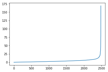
The first eigenvalue is as good as zero and this is a general fact; the smallest eigenvalue is always zero. The reason it’s not exactly zero above is because of computational accuracy.
So, we will omit the first eigenvector since it does not convey any information.
We also take a 32-dimensional subspace of the full vector space:

    embedding_size = 32
    v_0 = eigenvectors[:, order[0]]
    v = eigenvectors[:, order[1:(embedding_size+1)]]

A plot of the eigenvalue looks like the following:

    plt.plot(eigenvalues)

png
Let’s use t-SNE to visualize out 32-dimensional organization:

    tsne = TSNE()
    v_pr = tsne.fit_transform(v)
    alpha=0.7
    label_map = { l: i for i, l in enumerate(np.unique(node_targets))}
    node_colours = [ label_map[target] for target in node_targets]
    fig = plt.figure(figsize=(10,8))
    plt.scatter(v_pr[:,0],
                v_pr[:,1],
                c=node_colours, cmap="jet", alpha=alpha)

png
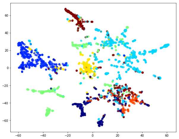
We see that the eigenvectors of the Laplacian form clusters corresponding to the target labels. It means that in principle we can train a model using the eigenvectors and make predictions about an unseen graphs. Simply said, given an unlabelled graph we can extract its Laplacian, feed it to the model and get labels for the nodes.

Training a classifier

The eigenvectors are from the point of view of machine learning just ordinary feature vectors. Taking a training and test set really means in this case taking a subset of the nodes (a subgraph) even though on a code level it’s just an ordinary classifier.

    X = v
    Y = np.array(node_targets)
    clf = RandomForestClassifier(n_estimators=10, min_samples_leaf=4)
    X_train, X_test, y_train, y_test = train_test_split(X, Y, train_size=140, random_state=42)
    clf.fit(X_train, y_train)
RandomForestClassifier(bootstrap=True, class_weight=None, criterion='gini',
            max_depth=None, max_features='auto', max_leaf_nodes=None,
            min_impurity_decrease=0.0, min_impurity_split=None,
            min_samples_leaf=4, min_samples_split=2,
            min_weight_fraction_leaf=0.0, n_estimators=10, n_jobs=None,
            oob_score=False, random_state=None, verbose=0,
            warm_start=False)
    print("score on X_train {}".format(clf.score(X_train, y_train)))
    print("score on X_test {}".format(clf.score(X_test, y_test)))
score on X_train 0.8571428571428571
score on X_test 0.7292110874200426

From here on you can experiment with different embedding dimensions, different Laplacians or any other matrix representing the structure of the graph.

To understand communities you best approach it via small datasets rather than big data. NetworkX is the ideal toolkit along the journey.

A graph database is one that stores data in terms of entities and the relationships between entities. A variant on this theme are RDF (resource description framework) databases which store data in the format subject-predicate-object, which is known as a triple.

There are three types of graph database: true graph databases, triple stores and conventional databases that provide some graphical capabilities. Triple stores are often referred to as RDF or semantic databases. The difference between a true graph product and a triple store is that the former supports index free adjacency (which means you can traverse a graph without needing an index) and the latter doesn’t. The former are designed to support property graphs (graphs where properties may be assigned to either entities or their relationships, or both) but recently some triple stores have added this capability.

Both graph and RDF databases may be native products or they may be built on top of other database types. Most commonly, other database types are forms of NoSQL database though there are some relational implementations.

RDF databases target semantic processing, often with the ability to combine information across structured and unstructured data. Both graph and RDF databases may be ACID compliant and both are frequently targeted at transactional environments. All graph products target analytics but different products are targeted at operational analytics (those suitable for transactional environments) as opposed to data warehousing analytics. In this last category there is also a distinction between vendors targeting known-known problems as opposed to those that also cover known-unknowns and those tackling unknown-unknowns: the most intractable of all.

Given that both graph and RDF databases target both transactional environments and have query processing capabilities, these are an obvious candidate for supporting so-called HTAP processing whereby the database is used for both transactional/operational processing and real-time analytics. Compared to some other approaches to HTAP this has the major advantage that the data only needs to be stored once. Both concurrent analytics (where the analytics is separate from operational processes, for example in supporting real-time dashboards) and in-process analytics (where the analytics are embedded in real-time operational processing) may be supported. In the latter case, there are a variety of graph 

algorithms supported by vendors that may be implemented for machine learning purposes.

Graph databases handle a class of issues that are too structured for NoSQL and too diverse for relational technologies. In the latter case, relational databases are inherently limited to one-to-one, many-to-one and one-to-many relationships. They do not cater well for problems (such as bill of materials – a classic case) that are many-to-many. For these types of requirements graph databases not only perform way better better than relational databases but they allow some types of query that are simply not possible otherwise. Semantic query support tends to be particularly strong in triple stores.

Another major point is that research suggests that graph visualisations are very easy and intuitive for users. It is also worth noting that many (not all) graph products are schema-free. This means that if you want to change the structure of the environment you simply add a new entity or relationship as required and do not have to explicitly implement a schema change. This is a major advantage over relational databases.

This market is emerging and there are many open source projects and vendors, many of which will not ultimately survive. Nevertheless there are still new products coming on to the marketplace. Conversely, there are companies that have been in this space for more than a decade, so the technology is not entirely new. One noticeable trend is for triple store vendors to add support for property graphs.

Another trend is towards multi-model implementations. This is where the database supports graph technology as just one of possibly several views into the data. A major consideration with such offerings is the extent to which these different representations can work together. Some vendors require, for example, require a different API to be used for each model type supported, whereas others have integrated their environment so that the different models are effectively transparent to one another.

One major issue that has yet to be finalised is with respect to language support. SPARQL (SPARQL protocol and RDF query language) is a W3C standard and is a declarative language but by no means all vendors support it. In general, RDF vendors support SPARQL, but property graph vendors do not, though there are exceptions to this. In the property graph space the 

Gremlin graph traversal language is part of the Apache Tinkerpop project and is supported by some vendors, while other suppliers have adopted their own “SQL-like” languages. Also with significant traction is OpenCypher, which is a declarative language (Gremlin is only partially so). ANSI has a working party to define SQL extensions to support graph processing while there is also an initiative to create a standardised GQL (graph query language). It is also worth noting that GraphQL, which is an open source project, is gaining traction as a graph API to replace REST.

Finally, while it is too early to call this trend one vendor has introduced a graph capability based on adjacency matrices rather than adjacency lists. If this proves successful, and early results suggest that that will be the case, then we are like to see this being more widely adopted as it promises much better performance.

There have been a lot of new entrants to the market and changes amongst those within the market. As far as new products are concerned these include RedisGraph, TigerGraph, MemGraph, Trovares, and Microsoft Cosmos DB. Cambridge Semantics has unbundled AnzoGraph from its Anzo Data Lake offering and both Amazon and SAP have also entered the market. In the case of Amazon Neptune, it is an open secret that this is based on BlazeGraph while SAP has acquired OrientDB. Or, rather, it acquired the company that had acquired OrientDB, though we think that OrientDB was probably incidental as far as this acquisition was concerned. Nevertheless, SAP appears to be moving ahead with the product though there is the perennial danger that it may increasingly be targeted at the SAP user base rather than the wider community.

The one company that has withdrawn from the graph space is IBM. However, the company continues to work on the development of JanusGraph (effectively a replacement to Titan).

Despite all of the above, the market leaders in this space continue to be Neo4J and OntoText (GraphDB), which are graph and RDF database providers respectively. These are the longest established vendors in this space (both founded in 2000) so they have a longevity and experience that other suppliers cannot yet match. How long this will remain the case remains to be seen.