Node2Vec with weighted random walks

This notebook illustrates how Node2Vec can be applied to learn low dimensional node embeddings of an edge weighted graph through weighted biased random walks over the graph.
The example uses components from the stellargraph, Gensim, and scikit-learn libraries.
The following references can be useful:

• Node2Vec: Scalable Feature Learning for Networks. A. Grover, J. Leskovec. ACM SIGKDD International Conference on Knowledge Discovery and Data Mining (KDD), 2016.
• Distributed representations of words and phrases and their compositionality. T. Mikolov, I. Sutskever, K. Chen, G. S. Corrado, and J. Dean. In Advances in Neural Information Processing Systems (NIPS), pp. 3111-3119, 2013.
• Gensim: Topic modelling for humans.
• scikit-learn: hardly needs an explanation.

Let’s import the necessary bits as usual. The most important one is Stellargraph:

    from sklearn.manifold import TSNE
    from sklearn.model_selection import train_test_split
    from sklearn.linear_model import LogisticRegressionCV
    from sklearn.metrics import accuracy_score
    from sklearn.metrics.pairwise import pairwise_distances
    from sklearn import preprocessing
    import os
    import networkx as nx
    import numpy as np
    import pandas as pd
    from stellargraph.data import BiasedRandomWalk
    from stellargraph import StellarGraph
    from gensim.models import Word2Vec
    import warnings
    import collections
    import matplotlib.pyplot as plt
    %matplotlib inline
Using TensorFlow backend.

The dataset is the citation Cora network. The Cora dataset consists of 2708 scientific publications classified into one of seven classes. The citation network consists of 5429 links. Each publication in the dataset is described by a 0/1-valued word vector indicating the absence/presence of the corresponding word from the dictionary. The dictionary consists of 1433 unique words. The README file in the dataset provides more details.
For this demo, we ignore the word vectors associated with each paper. We are only interested in the network structure and the subject attribute of each paper.
Download and unzip the cora.tgz file to a location on your computer, let’s assume it’s ~/data/cora/.

    data_dir = "~/data/cora"

Next, we create a normal undirected NetworkX graph:

    cora_location = os.path.expanduser(os.path.join(data_dir, "cora.cites"))
    g_nx_wt = nx.read_weighted_edgelist(path=cora_location, create_using=nx.DiGraph()).reverse()
    g_nx_wt = g_nx_wt.to_undirected()

Assign the ‘subject’ to the node:

    cora_data_location = os.path.expanduser(os.path.join(data_dir, "cora.content"))
    node_attr = pd.read_csv(cora_data_location, sep='\t', header=None)
    values = { str(row.tolist()[0]): row.tolist()[-1] for _, row in node_attr.iterrows()}
    nx.set_node_attributes(g_nx_wt, values, 'subject')

Select the largest connected component. For clarity we ignore isolated nodes and subgraphs; having these in the data does not prevent the algorithm from running and producing valid results.

    g_nx_wt = max(nx.connected_component_subgraphs(g_nx_wt, copy=True), key=len)
    print("Largest subgraph statistics: {} nodes, {} edges".format(
        g_nx_wt.number_of_nodes(), g_nx_wt.number_of_edges()))
Largest subgraph statistics: 2485 nodes, 5069 edges

For weighted biased random walks the underlying graph should have weights over the edges. Since the links in the Cora dataset are unweighted, we need to synthetically add weights to the links in the graph. One possibility is to weight each edge by the similarity of its end nodes. Here we assign the Jaccard similarity of the features of the pair of nodes as the weight of edge:

    df = node_attr.copy()
    df.set_index(0, inplace = True)
    papers = df.index
    ## calculating the paiwise jaccard similarity between each pair of nodes.
    with warnings.catch_warnings():
        warnings.simplefilter("ignore")
        wts = pd.DataFrame(
            1- pairwise_distances(df.iloc[:,:-1].values, metric = 'jaccard'),
            index = papers, columns = papers)
        wts.index = wts.index.map(str)
        wts.columns = wts.columns.map(str)

Append the weight attribute to the edges. Note, here we use the word ‘weight’ to label the weight value over the edge but it can be any other user specified label.

    for u,v in g_nx_wt.edges():
        val = wts[u][v]
        g_nx_wt[u][v]['weight'] = val

The weights distribution can be seen as follows:

    wts = list()
    for u,v in g_nx_wt.edges():
        wts.append(g_nx_wt[u][v]['weight'])
    wts = sorted(wts, reverse = True)
    edgeCount = collections.Counter(wts)
    wt, cnt = zip(*edgeCount.items())
    plt.figure(figsize=(10,8))
    plt.bar(wt, cnt, width=0.005, color='b')
    plt.title("Edge weights histogram")
    plt.ylabel("Count")
    plt.xlabel("edge weights")
    plt.xticks(np.linspace(0,1,10))
    plt.show()

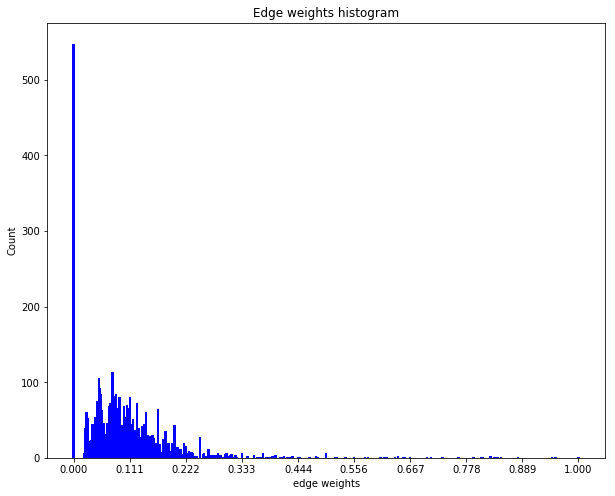
The above distribution of edge weights illustrates that majority of linked nodes are insignificantly similar in terms of their attributes.
The Node2Vec algorithm is a method for learning continuous feature respresentations for nodes in networks. This approach can simply be described as a mapping of nodes to a low dimensional space of features that maximizes the likelihood of preservering neighborhood sgrtucture of the nodes. This approach is not tied to a fixed definition of neighborhood of a node but can be used in conjunction with different notions of node neighborhood, such as, homophily or structural equivalence, among other concepts. The algorithm efficiently explores diverse neighborhoods of nodes through a biased random walk procedure that is parametrized to emulate a specific concept of the neighborhood of a node.
Once a pre-defined number of walks, of fixed lengths, have been sampled, the low dimension embedding vectors of nodes can be learnt using Word2vec algorithm. We use the Word2Vec implementation in the Gensim library but any other can do.
The Stellargraph library provides an implementation of random walks that can be unweighted or weighted as required by Node2Vec. The random walks have a pre-defined fixed maximum length and are controlled by three parameters p, q, and weight. By default, the weight over the edges is assumed to be 1.
The first step for the weighted biased random walk is to build a random walk object by passing it a Stellargraph object.

    rw = BiasedRandomWalk(StellarGraph(g_nx_wt))

The next step is to sample a set of random walks of pre-defined length starting from each node of the graph. Parameters p, q, and weighted influence the type of random walks in the procedure. In this demo, we are going to start 10 random walks from each node in the graph with a length up to 100. We set parameter p to 0.5 and q to 2.0 and the weight parameter set to True. The run method in the random walk will check if the weights over the edges are available and resolve other issues, such as, whether the weights are numeric and that their is no ambiguity of edge traversal (i.e. each pair of node is connected by a unique numerically weighted edge).

    weighted_walks = rw.run(
        nodes=g_nx_wt.nodes(), # root nodes
        length=100,    # maximum length of a random walk
        n=10,          # number of random walks per root node
        p=0.5,         # Defines (unormalised) probability, 1/p, of returning to source node
        q=2.0,         # Defines (unormalised) probability, 1/q, for moving away from source node
        weighted=True, #for weighted random walks
        seed=42        # random seed fixed for reproducibility
    )
    print("Number of random walks: {}".format(len(weighted_walks)))
Number of random walks: 24850

Once we have a sample set of walks, we learn the low-dimensional embedding of nodes using Word2Vec approach.
We set the dimensionality of the learned embedding vectors to 128.

    weighted_model = Word2Vec(weighted_walks, size=128, window=5, min_count=0, sg=1, workers=1, iter=1)

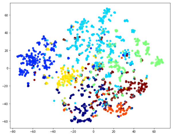
To visualise node embeddings generated by weighted random walks we can use t-SNE.
We retrieve the Word2Vec node embeddings that are 128-dimensional vectors and then we project them down to 2 dimensions using the t-SNE algorithm for visualization.

    # Retrieve node embeddings and corresponding subjects
    node_ids = weighted_model.wv.index2word  # list of node IDs
    weighted_node_embeddings = weighted_model.wv.vectors  # numpy.ndarray of size number of nodes times embeddings dimensionality
    node_targets = [ g_nx_wt.node[node_id]['subject'] for node_id in node_ids]
    # Apply t-SNE transformation on node embeddings
    tsne = TSNE(n_components=2 , random_state=42)
    weighted_node_embeddings_2d = tsne.fit_transform(weighted_node_embeddings)

The values of weighted_node_embeddings_2d can be plotted:

    # draw the points
    alpha = 0.7
    label_map = {l: i for i, l in enumerate(np.unique(node_targets))}
    node_colours = [ label_map[target] for target in node_targets ]
    plt.figure(figsize=(10,8))
    plt.scatter(weighted_node_embeddings_2d[:,0],
                weighted_node_embeddings_2d[:,1],
                c=node_colours, cmap = "jet", alpha = 0.7)
    plt.show()

The node embeddings calculated using Word2Vec can be used as feature vectors in a downstream task such as node classification. Here we give an example of training a logistic regression classifier using the node embeddings, learnt above, as features.

    X = weighted_node_embeddings
    y = np.array(node_targets)

Note that you can mix embedding values and standard feature values in the full feature vector.
We use 75% of the data for training and the remaining 25% for testing as a hold out test set.

    X_train, X_test, y_train, y_test = train_test_split(
        X, y, train_size=0.75, test_size=None, random_state = 42
    )
    print("Array shapes:\n X_train = {}\n y_train = {}\n X_test = {}\n y_test = {}" \
          .format(X_train.shape, y_train.shape, X_test.shape, y_test.shape))
Array shapes:
 X_train = (1863, 128)
 y_train = (1863,)
 X_test = (622, 128)
 y_test = (622,)

A logistic regression is learned:

    clf = LogisticRegressionCV(
        Cs=10,
        cv=10,
        tol=0.001,
        max_iter=1000,
        scoring="accuracy",
        verbose=False,
        multi_class='ovr',
        random_state=5434
    )
    clf.fit(X_train, y_train)
LogisticRegressionCV(Cs=10, class_weight=None, cv=10, dual=False,
           fit_intercept=True, intercept_scaling=1.0, max_iter=1000,
           multi_class='ovr', n_jobs=None, penalty='l2', random_state=5434,
           refit=True, scoring='accuracy', solver='lbfgs', tol=0.001,
           verbose=False)

and, as always, we predict things to evaluate the accuracy of the model:

    y_pred = clf.predict(X_test)
    accuracy_score(y_test, y_pred)
0.8135048231511254

Comparison of weighted and unnweighted biased random walks

Lets compare weighted random walks with unweighted random walks. This simply requires toggling the weight parameter to False in the run method of the BiasedRandomWalk. Note, the weight parameter is by default set to False, hence, not specifying the weight parameter would result in the same action.

    walks = rw.run(
        nodes=g_nx_wt.nodes(), # root nodes
        length=100,     # maximum length of a random walk
        n=10,           # number of random walks per root node
        p=0.5,          # Defines (unormalised) probability, 1/p, of returning to source node
        q=2.0,          # Defines (unormalised) probability, 1/q, for moving away from source node
        weighted=False, # since we are interested in unweighted walks
        seed=42         # for reproducibility
    )
    print("Number of random walks: {}".format(len(walks)))
    model = Word2Vec(walks, size=128, window=5, min_count=0, sg=1, workers=1, iter=1)
Number of random walks: 24850

We use the same t-SNE trick to plot the embedding:

    # Retrieve node embeddings and corresponding subjects
    node_ids = model.wv.index2word  # list of node IDs
    node_embeddings = model.wv.vectors  # numpy.ndarray of size number of nodes times embeddings dimensionality
    node_targets = [ g_nx_wt.node[node_id]['subject'] for node_id in node_ids]
    # Apply t-SNE transformation on node embeddings
    tsne = TSNE(n_components=2, random_state=42)
    node_embeddings_2d = tsne.fit_transform(node_embeddings)
    # draw the points
    alpha = 0.7
    label_map = { l: i for i, l in enumerate(np.unique(node_targets))}
    node_colours = [ label_map[target] for target in node_targets]
    plt.figure(figsize=(10,8))
    plt.scatter(node_embeddings_2d[:,0],
                node_embeddings_2d[:,1],
                c=node_colours, cmap = "jet", alpha = 0.7)
    plt.show()

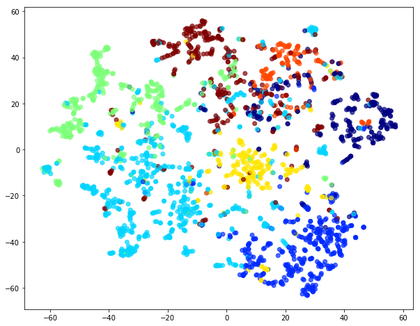
Visual comparison of node embedding plots for weighted and unweighted random walks illustrates the differences betweem the two.
Going a step further, we can see how the unweighted approach predicts things.

    # X will hold the 128-dimensional input features
    X = node_embeddings
    # y holds the corresponding target values
    y = np.array(node_targets)
    X_train, X_test, y_train, y_test = train_test_split(
        X, y, train_size=0.75, test_size=None, random_state=42
    )
    clf = LogisticRegressionCV(
        Cs=10,
        cv=10,
        tol=0.01,
        max_iter=1000,
        scoring="accuracy",
        verbose=False,
        multi_class='ovr',
        random_state=5434
    )
    clf.fit(X_train, y_train)
    y_pred = clf.predict(X_test)
    accuracy_score(y_test, y_pred)
0.8520900321543409

Generally, the node embeddings extracted from unweighted random walks are more representative of the underlying community structure of the Cora dataset than the embeddings learnt from weighted random walks over the artificially weighted Cora network.
Of course, this is not a general statement. Also note that we assigned weights in a particular synthetic fashion. If the weights are given the accuracy could be higher.

Testing whether weights = 1 gives identical result to unweighted randomwalks

Lastly, we demonstrate that weighted biased random walks are identical to unweighted biased random walks when weights over the edges are identically 1.
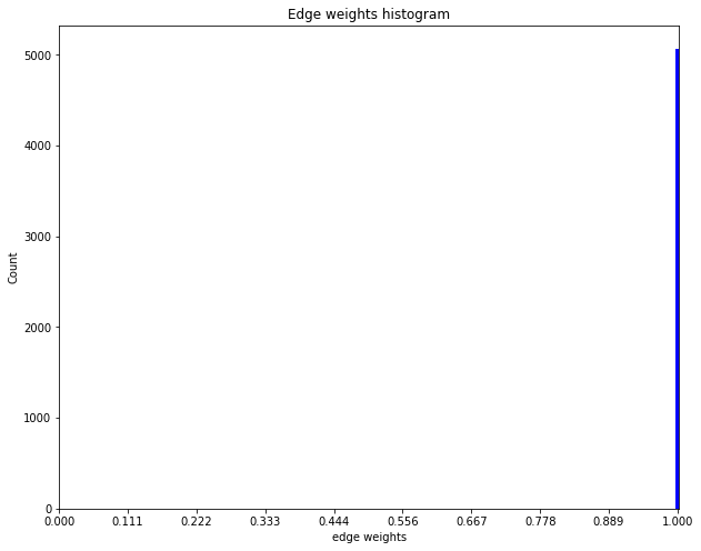
First, set weights of all edges in the graph to 1.

    for u,v in g_nx_wt.edges():
        g_nx_wt[u][v]['weight'] = 1

Quick check to confirm if all edge weights are actually 1.

    wts = list()
    for u,v in g_nx_wt.edges():
        wts.append(g_nx_wt[u][v]['weight'])
    wts = sorted(wts, reverse = True)
    edgeCount = collections.Counter(wts)
    wt, cnt = zip(*edgeCount.items())
    plt.figure(figsize=(10,8))
    plt.bar(wt, cnt, width=0.005, color='b')
    plt.title("Edge weights histogram")
    plt.ylabel("Count")
    plt.xlabel("edge weights")
    plt.xticks(np.linspace(0,1,10))
    plt.show()

    rw = BiasedRandomWalk(StellarGraph(g_nx_wt))
    weighted_walks = rw.run(
        nodes=g_nx_wt.nodes(), # root nodes
        length=100,    # maximum length of a random walk
        n=10,          # number of random walks per root node
        p=0.5,         # Defines (unormalised) probability, 1/p, of returning to source node
        q=2.0,         # Defines (unormalised) probability, 1/q, for moving away from source node
        weighted=True, # indicates the walks are weighted
        seed=42        # seed fixed for reproducibility
    )
    print("Number of random walks: {}".format(len(weighted_walks)))
Number of random walks: 24850

Compare unweighted walks with weighted walks when all weights are uniformly set to 1. Note, the two sets should be identical given all other parameters and random seeds are fixed.

    assert walks == weighted_walks
    weighted_model = Word2Vec(weighted_walks, size=128, window=5, min_count=0, sg=1, workers=1, iter=1)

If you once again plot the embedding you can see that unweighted and weight one embeddings are identical.

    # Retrieve node embeddings and corresponding subjects
    node_ids = weighted_model.wv.index2word  # list of node IDs
    weighted_node_embeddings = weighted_model.wv.vectors  # numpy.ndarray of size number of nodes times embeddings dimensionality
    node_targets = [ g_nx_wt.node[node_id]['subject'] for node_id in node_ids]
    # Apply t-SNE transformation on node embeddings
    tsne = TSNE(n_components=2, random_state=42)
    weighted_node_embeddings_2d = tsne.fit_transform(weighted_node_embeddings)
    # draw the points
    alpha = 0.7
    label_map = { l: i for i, l in enumerate(np.unique(node_targets))}
    node_colours = [ label_map[target] for target in node_targets]
    plt.figure(figsize=(10,8))
    plt.scatter(weighted_node_embeddings_2d[:,0],
                weighted_node_embeddings_2d[:,1],
                c=node_colours, cmap = "jet", alpha = 0.7)
    plt.show()

Compare classification of nodes through logistic regression on embeddings learnt from weighted (weight == 1) walks to that of unweighted walks demonstrated above.

    # X will hold the 128-dimensional input features
    X = weighted_node_embeddings
    # y holds the corresponding target values
    y = np.array(node_targets)
    X_train, X_test, y_train, y_test = train_test_split(
        X, y, train_size=0.75, test_size=None, random_state=42
    )
    print("Array shapes:\n X_train = {}\n y_train = {}\n X_test = {}\n y_test = {}" \
          .format(X_train.shape, y_train.shape, X_test.shape, y_test.shape))
Array shapes:
 X_train = (1863, 128)
 y_train = (1863,)
 X_test = (622, 128)
 y_test = (622,)
    clf = LogisticRegressionCV(
        Cs=10,
        cv=10,
        tol=0.001,
        max_iter=1000,
        scoring="accuracy",
        verbose=False,
        multi_class='ovr',
        random_state=5434
    )
    clf.fit(X_train, y_train)
    y_pred = clf.predict(X_test)
    accuracy_score(y_test, y_pred)
    np.array_equal(weighted_node_embeddings, node_embeddings)
True

The weighted random walks with weight == 1 are identical to unweighted random walks. Moreover, the embeddings learnt over the two kinds of walks are identical as well.