In a previous article we explained how GraphSage can be used for link predictions. This article shows that the same method can be used to make predictions on a node level.
The research paper is the same as for link predictions, that is “Inductive Representation Learning on Large Graphs”. Also, like pretty much all graph learning articles on this site, we’ll use the Cora dataset.
Purpose of this article is to show that the ‘subject’ of each paper in the Cora graph can be predicted on the basis of the graph structure together with whatever features are additionally available on the nodes.
    import networkx as nx
    import pandas as pd
    import os
    import stellargraph as sg
    from stellargraph.mapper import GraphSAGENodeGenerator
    from stellargraph.layer import GraphSAGE
    # note that using "from keras" will not work
    from tensorflow.keras import layers, optimizers, losses, metrics, Model
    from sklearn import preprocessing, feature_extraction, model_selection
Data import
Please read through our Cora dataset article to understand a bit what the following code does:
    data_dir = os.path.expanduser("~/data/cora")
    cora_location = os.path.expanduser(os.path.join(data_dir, "cora.cites"))
    g_nx = nx.read_edgelist(path=cora_location)
    cora_data_location = os.path.expanduser(os.path.join(data_dir, "cora.content"))
    node_attr = pd.read_csv(cora_data_location, sep='\t', header=None)
    values = { str(row.tolist()[0]): row.tolist()[-1] for _, row in node_attr.iterrows()}
    nx.set_node_attributes(g_nx, values, 'subject')
    g_nx_ccs = (g_nx.subgraph(c).copy() for c in nx.connected_components(g_nx))
    g_nx = max(g_nx_ccs, key=len)
    feature_names = ["w_{}".format(ii) for ii in range(1433)]
    column_names =  feature_names + ["subject"]
    node_data = pd.read_csv(os.path.join(data_dir, "cora.content"), header=None, names=column_names, sep='\t')
    node_data.index = node_data.index.map(str)
    node_data = node_data[node_data.index.isin(list(g_nx.nodes()))]
The ‘subject’ label on the nodes is what we’ll learn and predict:
    set(node_data["subject"])
{'Case_Based',
 'Genetic_Algorithms',
 'Neural_Networks',
 'Probabilistic_Methods',
 'Reinforcement_Learning',
 'Rule_Learning',
 'Theory'}
Splitting the data
The GraphSage generator takes the graph structure and the node-data as input and can then be used in a Keras model like any other data generator. The indices we give to the generator also defines which nodes will be used to train the model. So, we can split the node-data in a training and testing set like any other dataset and use the indices as a reference to what belongs to which datasets.
train_data, test_data = model_selection.train_test_split(node_data, train_size=0.1, test_size=None, stratify=node_data['subject'], random_state=42)
The features are all numeric but the targets are now, so we use a standard one-hot encoding:
    target_encoding = feature_extraction.DictVectorizer(sparse=False)
    train_targets = target_encoding.fit_transform(train_data[["subject"]].to_dict('records'))
    test_targets = target_encoding.transform(test_data[["subject"]].to_dict('records'))
    node_features = node_data[feature_names]
    node_features.head(2)
| w_0 | w_1 | w_2 | w_3 | w_4 | w_5 | w_6 | w_7 | w_8 | w_9 | w_10 | w_11 | w_12 | w_13 | w_14 | w_15 | w_16 | w_17 | w_18 | w_19 | w_20 | w_21 | w_22 | w_23 | w_24 | w_25 | w_26 | w_27 | w_28 | w_29 | w_30 | w_31 | w_32 | w_33 | w_34 | w_35 | w_36 | w_37 | w_38 | w_39 | … | w_1393 | w_1394 | w_1395 | w_1396 | w_1397 | w_1398 | w_1399 | w_1400 | w_1401 | w_1402 | w_1403 | w_1404 | w_1405 | w_1406 | w_1407 | w_1408 | w_1409 | w_1410 | w_1411 | w_1412 | w_1413 | w_1414 | w_1415 | w_1416 | w_1417 | w_1418 | w_1419 | w_1420 | w_1421 | w_1422 | w_1423 | w_1424 | w_1425 | w_1426 | w_1427 | w_1428 | w_1429 | w_1430 | w_1431 | w_1432 | |
|---|---|---|---|---|---|---|---|---|---|---|---|---|---|---|---|---|---|---|---|---|---|---|---|---|---|---|---|---|---|---|---|---|---|---|---|---|---|---|---|---|---|---|---|---|---|---|---|---|---|---|---|---|---|---|---|---|---|---|---|---|---|---|---|---|---|---|---|---|---|---|---|---|---|---|---|---|---|---|---|---|---|
| 31336 | 0 | 0 | 0 | 0 | 0 | 0 | 0 | 0 | 0 | 0 | 0 | 0 | 0 | 0 | 0 | 0 | 0 | 0 | 0 | 0 | 0 | 0 | 0 | 0 | 0 | 0 | 0 | 0 | 0 | 0 | 0 | 0 | 0 | 0 | 0 | 0 | 0 | 0 | 0 | 0 | … | 0 | 0 | 0 | 0 | 0 | 0 | 0 | 0 | 0 | 0 | 0 | 0 | 0 | 0 | 0 | 0 | 0 | 0 | 0 | 0 | 0 | 0 | 0 | 0 | 0 | 0 | 0 | 0 | 0 | 0 | 0 | 0 | 0 | 1 | 0 | 0 | 0 | 0 | 0 | 0 |
| 1061127 | 0 | 0 | 0 | 0 | 0 | 0 | 0 | 0 | 0 | 0 | 0 | 0 | 1 | 0 | 0 | 0 | 0 | 0 | 0 | 0 | 0 | 0 | 0 | 0 | 0 | 0 | 0 | 0 | 0 | 0 | 0 | 0 | 0 | 0 | 0 | 0 | 0 | 0 | 0 | 0 | … | 0 | 0 | 0 | 0 | 0 | 0 | 0 | 0 | 0 | 0 | 0 | 0 | 0 | 0 | 0 | 0 | 0 | 0 | 0 | 0 | 0 | 0 | 0 | 0 | 0 | 0 | 0 | 0 | 0 | 0 | 0 | 0 | 1 | 0 | 0 | 0 | 0 | 0 | 0 | 0 |
2 rows × 1433 columns
The Keras model
The graph structure (a NetworkX graph) is turned into a StellarGraph:
G = sg.StellarGraph(g_nx, node_features=node_features)
Next, we create a generator which later on will be used by a Keras model to load the data in batches. Besides the batch size you also need to specify the layers. The documentation explains it well:
    help(GraphSAGENodeGenerator)
Help on class GraphSAGENodeGenerator in module stellargraph.mapper.node_mappers:
class GraphSAGENodeGenerator(builtins.object)
 |  GraphSAGENodeGenerator(G, batch_size, num_samples, schema=None, seed=None, name=None)
 |
 |  A data generator for node prediction with Homogeneous GraphSAGE models
 |
 |  At minimum, supply the StellarGraph, the batch size, and the number of
 |  node samples for each layer of the GraphSAGE model.
 |
 |  The supplied graph should be a StellarGraph object that is ready for
 |  machine learning. Currently the model requires node features for all
 |  nodes in the graph.
 |
 |  Use the :meth:`flow` method supplying the nodes and (optionally) targets
 |  to get an object that can be used as a Keras data generator.
 |
 |  Example::
 |
 |      G_generator = GraphSAGENodeGenerator(G, 50, [10,10])
 |      train_data_gen = G_generator.flow(train_node_ids, train_node_labels)
 |      test_data_gen = G_generator.flow(test_node_ids)
 |
 |  Args:
 |      G (StellarGraph): The machine-learning ready graph.
 |      batch_size (int): Size of batch to return.
 |      num_samples (list): The number of samples per layer (hop) to take.
 |      schema (GraphSchema): [Optional] Graph schema for G.
 |      seed (int): [Optional] Random seed for the node sampler.
 |      name (str or None): Name of the generator (optional)
 |
 |  Methods defined here:
 |
 |  __init__(self, G, batch_size, num_samples, schema=None, seed=None, name=None)
 |      Initialize self.  See help(type(self)) for accurate signature.
 |
 |  flow(self, node_ids, targets=None, shuffle=False)
 |      Creates a generator/sequence object for training or evaluation
 |      with the supplied node ids and numeric targets.
 |
 |      The node IDs are the nodes to train or inference on: the embeddings
 |      calculated for these nodes are passed to the downstream task. These
 |      are a subset of the nodes in the graph.
 |
 |      The targets are an array of numeric targets corresponding to the
 |      supplied node_ids to be used by the downstream task. They should
 |      be given in the same order as the list of node IDs.
 |      If they are not specified (for example, for use in prediction),
 |      the targets will not be available to the downstream task.
 |
 |      Note that the shuffle argument should be True for training and
 |      False for prediction.
 |
 |      Args:
 |          node_ids: an iterable of node IDs
 |          targets: a 2D array of numeric targets with shape
 |              `(len(node_ids), target_size)`
 |          shuffle (bool): If True the node_ids will be shuffled at each
 |              epoch, if False the node_ids will be processed in order.
 |
 |      Returns:
 |          A NodeSequence object to use with the GraphSAGE model
 |          in Keras methods ``fit_generator``, ``evaluate_generator``,
 |          and ``predict_generator``
 |
 |  flow_from_dataframe(self, node_targets, shuffle=False)
 |      Creates a generator/sequence object for training or evaluation
 |      with the supplied node ids and numeric targets.
 |
 |      Args:
 |          node_targets: a Pandas DataFrame of numeric targets indexed
 |              by the node ID for that target.
 |          shuffle (bool): If True the node_ids will be shuffled at each
 |              epoch, if False the node_ids will be processed in order.
 |
 |      Returns:
 |          A NodeSequence object to use with the GraphSAGE model
 |          in Keras methods ``fit_generator``, ``evaluate_generator``,
 |          and ``predict_generator``
 |
 |  sample_features(self, head_nodes, sampling_schema)
 |      Sample neighbours recursively from the head nodes, collect the features of the
 |      sampled nodes, and return these as a list of feature arrays for the GraphSAGE
 |      algorithm.
 |
 |      Args:
 |          head_nodes: An iterable of head nodes to perform sampling on.
 |          sampling_schema: The sampling schema for the model
 |
 |      Returns:
 |          A list of the same length as ``num_samples`` of collected features from
 |          the sampled nodes of shape:
 |          ``(len(head_nodes), num_sampled_at_layer, feature_size)``
 |          where num_sampled_at_layer is the cumulative product of `num_samples`
 |          for that layer.
 |
 |  ----------------------------------------------------------------------
 |  Data descriptors defined here:
 |
 |  __dict__
 |      dictionary for instance variables (if defined)
 |
 |  __weakref__
 |      list of weak references to the object (if defined)
    batch_size = 50; num_samples = [10,20,10]
    generator = GraphSAGENodeGenerator(G, batch_size, num_samples)
For training we map only the training nodes returned from our splitter and the target values.
train_gen = generator.flow(train_data.index, train_targets)
The GraphSage model has a few parameters we need to specify:
layer_size: a list of hidden feature sizes of each layer in the model. More and bigger layers allow for better predictions but also overfitting. Not different from classic machine learning.biasanddropoutare aslo well-known from non-graph ML models.graphsage_model = GraphSAGE( layer_sizes=[32,32,32], generator=train_gen, bias=True, dropout=0.5, )
Now we create a model to predict the 7 categories using Keras softmax layers. Note that we need to use the G.get_target_size method to find the number of categories in the data.
    x_inp, x_out = graphsage_model.default_model(flatten_output=True)
    prediction = layers.Dense(units=train_targets.shape[1], activation="softmax")(x_out)
    prediction.shape
TensorShape([Dimension(None), Dimension(7)])
Training the model
Let’s create the actual Keras model with the graph inputs x_inp provided by the graph_model and outputs being the predictions from the softmax layer
    model = Model(inputs=x_inp, outputs=prediction)
    model.compile(
        optimizer=optimizers.Adam(lr=0.005),
        loss=losses.categorical_crossentropy,
        metrics=["acc"],
    )
Train the model, keeping track of its loss and accuracy on the training set, and its generalisation performance on the test set (we need to create another generator over the test data for this)
    test_gen = generator.flow(test_data.index, test_targets)
    history = model.fit_generator(
        train_gen,
        epochs=20,
        validation_data=test_gen,
        verbose=2,
        shuffle=True,
    )
Epoch 1/20
45/45 [==============================] - 79s 2s/step - loss: 1.7728 - acc: 0.2964
 - 89s - loss: 1.8732 - acc: 0.2903 - val_loss: 1.7728 - val_acc: 0.2964
Epoch 2/20
45/45 [==============================] - 78s 2s/step - loss: 1.6414 - acc: 0.4059
 - 86s - loss: 1.7473 - acc: 0.3629 - val_loss: 1.6414 - val_acc: 0.4059
Epoch 3/20
45/45 [==============================] - 77s 2s/step - loss: 1.5004 - acc: 0.6133
 - 84s - loss: 1.6111 - acc: 0.4758 - val_loss: 1.5004 - val_acc: 0.6133
Epoch 4/20
45/45 [==============================] - 76s 2s/step - loss: 1.3520 - acc: 0.6647
 - 82s - loss: 1.4646 - acc: 0.6331 - val_loss: 1.3520 - val_acc: 0.6647
Epoch 5/20
45/45 [==============================] - 75s 2s/step - loss: 1.2450 - acc: 0.7103
 - 82s - loss: 1.3431 - acc: 0.7460 - val_loss: 1.2450 - val_acc: 0.7103
Epoch 6/20
...
Epoch 20/20
45/45 [==============================] - 102s 2s/step - loss: 0.6952 - acc: 0.8136
 - 112s - loss: 0.3403 - acc: 0.9839 - val_loss: 0.6952 - val_acc: 0.8136
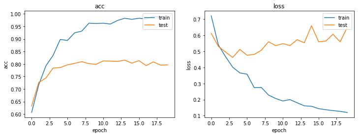
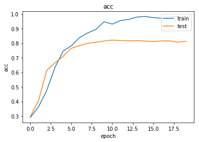
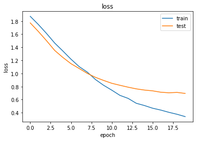
As always, use the history to plot the loss and accuracy over time:
    import matplotlib.pyplot as plt
    %matplotlib inline
    def plot_history(history):
        metrics = sorted(history.history.keys())
        metrics = metrics[:len(metrics)//2]
        for m in metrics:
            plt.plot(history.history[m])
            plt.plot(history.history['val_' + m])
            plt.title(m)
            plt.ylabel(m)
            plt.xlabel('epoch')
            plt.legend(['train', 'test'], loc='upper right')
            plt.show()
    plot_history(history)
Now we have trained the model we can evaluate on the test set.
    test_metrics = model.evaluate_generator(test_gen)
    print("\nTest Set Metrics:")
    for name, val in zip(model.metrics_names, test_metrics):
        print("\t{}: {:0.4f}".format(name, val))
Test Set Metrics:
    loss: 0.7049
    acc: 0.8087
Like any other ML task you can spend the rest of your life fine-tuning the model in zillion ways.
Making predictions with the model
Let’s see what gives when we predict all of the node labels:
    all_nodes = node_data.index
    all_mapper = generator.flow(all_nodes)
    all_predictions = model.predict_generator(all_mapper)
    # invert the one-hot encoding
    node_predictions = target_encoding.inverse_transform(all_predictions)
    results = pd.DataFrame(node_predictions, index=all_nodes).idxmax(axis=1)
    df = pd.DataFrame({"Predicted": results, "True": node_data['subject']})
    df.head(10)
| Predicted | True | |
|---|---|---|
| 31336 | subject=Theory | Neural_Networks |
| 1061127 | subject=Rule_Learning | Rule_Learning |
| 1106406 | subject=Reinforcement_Learning | Reinforcement_Learning |
| 13195 | subject=Reinforcement_Learning | Reinforcement_Learning |
| 37879 | subject=Probabilistic_Methods | Probabilistic_Methods |
| 1126012 | subject=Probabilistic_Methods | Probabilistic_Methods |
| 1107140 | subject=Theory | Theory |
| 1102850 | subject=Theory | Neural_Networks |
| 31349 | subject=Theory | Neural_Networks |
| 1106418 | subject=Theory | Theory |
We’ll augment the graph with the true vs. predicted label for visualization purposes:
    for nid, pred, true in zip(df.index, df["Predicted"], df["True"]):
        g_nx.node[nid]["subject"] = true
        g_nx.node[nid]["PREDICTED_subject"] = pred.split("=")[-1]
Also add isTrain and isCorrect node attributes:
    for nid in train_data.index:
        g_nx.node[nid]["isTrain"] = True
    for nid in test_data.index:
        g_nx.node[nid]["isTrain"] = False
    for nid in g_nx.nodes():
        g_nx.node[nid]["isCorrect"] = g_nx.node[nid]["subject"] == g_nx.node[nid]["PREDICTED_subject"]
To get an idea of how the prediction errors are distributed visually we’ll load the graph in yEd Live and apply a radial layout:
    pred_fname = "pred_n={}.graphml".format(num_samples)
    nx.write_graphml(g_nx,'~/nodepredictions.graphml')
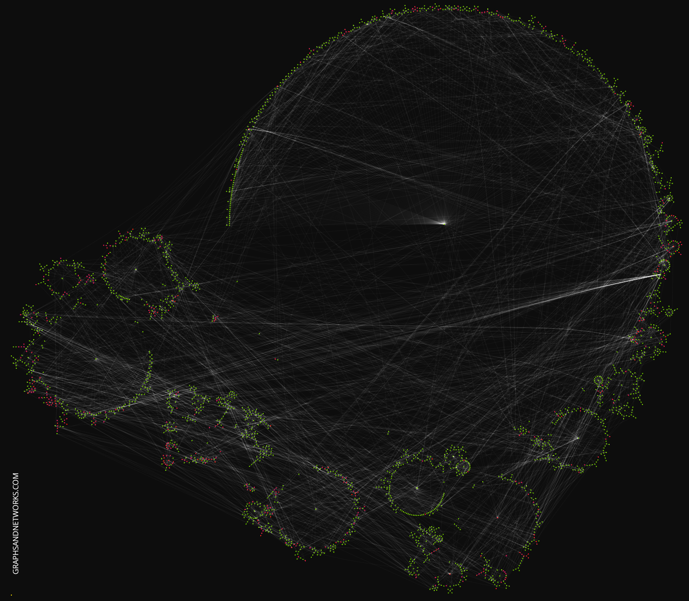
You can play with the graph in yEd Live, this link will load the graph directly.
What causes the errors? Is there a particular local topology giving rise to errors? Or is it solely the node features?
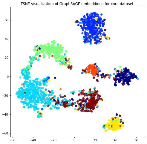
Node embeddings
Evaluate node embeddings as activations of the output of graphsage layer stack, and visualise them, coloring nodes by their subject label.
The GraphSAGE embeddings are the output of the GraphSAGE layers, namely the x_out variable. Let’s create a new model with the same inputs as we used previously x_inp but now the output is the embeddings rather than the predicted class. Additionally note that the weights trained previously are kept in the new model.
    embedding_model = Model(inputs=x_inp, outputs=x_out)
    emb = embedding_model.predict_generator(all_mapper)
    emb.shape
(2485, 32)
Project the embeddings to 2d using either TSNE or PCA transform, and visualise, coloring nodes by their subject label
    from sklearn.manifold import TSNE
    import pandas as pd
    import numpy as np
    X = emb
    y = np.argmax(target_encoding.transform(node_data[["subject"]].to_dict('records')), axis=1)
    if X.shape[1] > 2:
        transform = TSNE
        trans = transform(n_components=2)
        emb_transformed = pd.DataFrame(trans.fit_transform(X), index=node_data.index)
        emb_transformed['label'] = y
    else:
        emb_transformed = pd.DataFrame(X, index=node_data.index)
        emb_transformed = emb_transformed.rename(columns = {'0':0, '1':1})
        emb_transformed['label'] = y
    alpha = 0.7
    fig, ax = plt.subplots(figsize=(8,8))
    ax.scatter(emb_transformed[0], emb_transformed[1], c=emb_transformed['label'].astype("category"),
                cmap="jet", alpha=alpha)
    #ax.set(aspect="equal", xlabel="$X_1$", ylabel="$X_2$")
    plt.title('{} visualization of GraphSAGE embeddings for cora dataset'.format(transform.__name__))
    plt.show()