This is an overview of the many ways in which one can create graphs in Mathematica. It demonstrates the ubiquity of graphs and how Mathematica makes it easy to experiment with ideas. At the same time, various Mathematica symbols and techniques are presented which we will cover more in depth in later article.

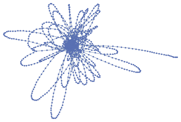
Polyhedral surfaces have been around since antiquity although it wasn’t recognized until Euler that they are in fact closely related to graphs. Take for example the snub-cube

and unwrap its faces

The number of vertices can be found in two ways here, either using the VertexCount property of the PolyHedronData or through the VertexCount property of Graph. The results do not agree though

because the vertex count of the polyhedron is based on its 3D wrapping while the unwrapped graph duplicates some vertices.

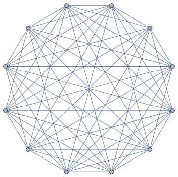
Polyhedrons can be combined to give beautiful graphics

The vertices in this case are contained in two graphs, we can use the GraphUnion command to combine them and thus create a new graph. The letter g will be used in this text to denote a graph.

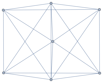
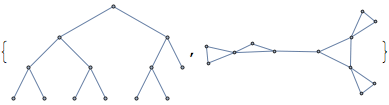
Turning this graph into a polyhedron is not possible (in a straightforward manner)but we can turn it into a 3d graph, which reveals that it’s almost a tree.

How far away from a tree? That’s something we can answer by looking at spanning trees. Although a spanning tree is not unique it still gives a good indication of how many edges (shortcuts) break the tree-like structure

A more numerical value can be obtained from the GraphDifference;

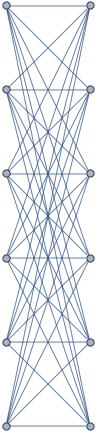
Once you have a graph there are many ways in which it can be turned into another graph. For example, a line graph of a given graph turns edges into vertices and vice versa;

Being a transformation, one can wonder whether there are graphs which remain invariant under this type of transformation. It’s rather easy to create a simple case, the triangle graph is indeed topologically invariant

and this is true for any cycle graph. Assuming that the symmetry of this graph is the key to invariance is misleading though

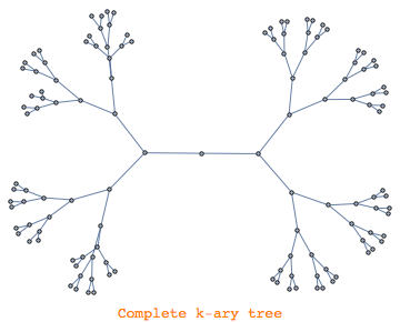
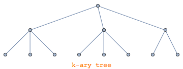
and similarly with k-ary trees

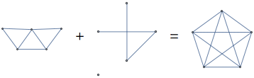
Another way to transform a graph into another one is by asking what it takes to turn the given graph into a complete one. Say, we take a random graph of 5 vertices and 7 edges

and take the graph complement

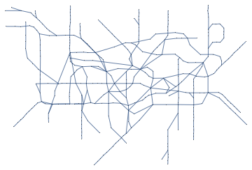
Graphs can be found everywhere in everyday life although it’s not always perceived as such. Millions of people traverse the London tube every day without realizing they do;

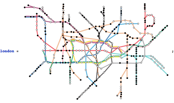
What is the longest trajectory across the London underground? One way to answer this question is by looking at the distance matrix

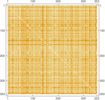
This gives a qualitative result and highlights a few regions with long distances. To find a qualitative answer we take the maximum

This corresponds to the so-called graph diameter, defined as the largest distance across the graph (using geodesic paths);

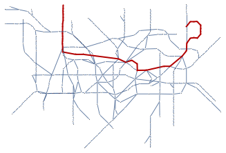
Of course, we want to know to which couple of stations this distance corresponds

which is a unique solution but can, of course, be traversed in two ways

So, let’s take the first one and see what the (shortest) path is connecting them

The explicit route is hence

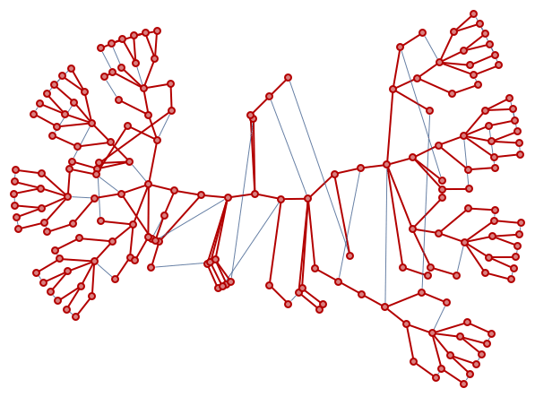
To represent this in the graph we first simplify the London graph somewhat.

and then highlight the longest path

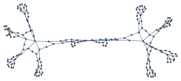
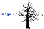
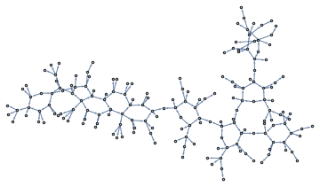
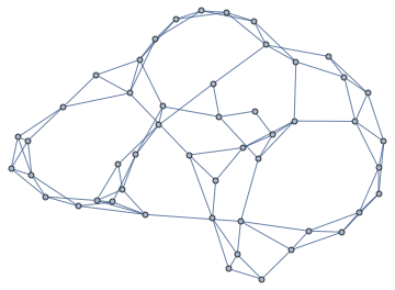
Graphs can be obtained from images through mathematical morphology. The following picture of a tree, for instance, can be turned into a tree-ish graph

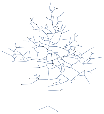
This indeed looks very much like a tree, but looks can be misleading;

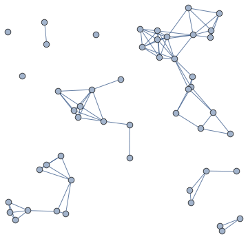
We can turn this into a genuine tree as follows

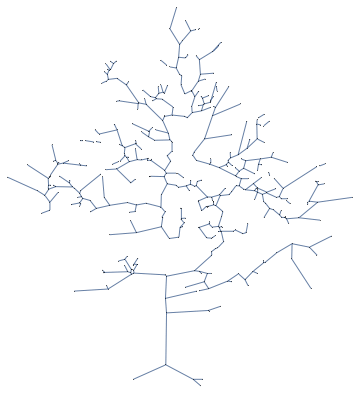
It’s actually not a tree but rather a forest, i.e. a collection of trees. This can be seen in various ways. If we apply a tree layout to the graph

we see that there are multiple components. This can be seen by using the ConnectedComponents and the ConnectedGraphQ methods as well

Is connected: False

The world of chemistry also offersa rich collection of graphs. For example, digitonin is a detergent

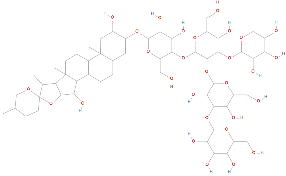
This molecular structure can be converted to a graph by fetching the edge collection

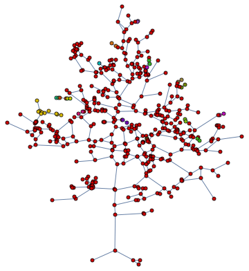
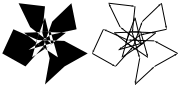
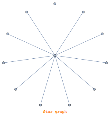
Mathematica has a rich collection of curated graphs and a fun way to explore a random sample is by means of

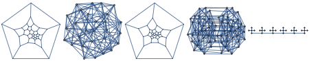
There are plenty of categorizations which one can focus on

The polyhedral graphs can be sampled in a similar way

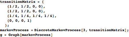
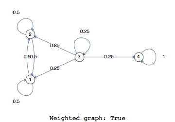
Markov processes can be modelled in Mathematica and their graph representation help understand visually the transitions

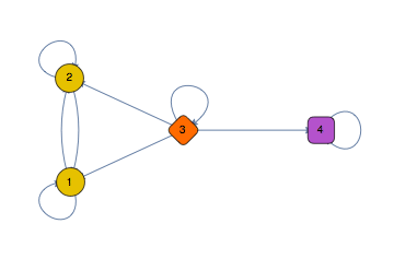
This graphical representation does not show the graph as a weighted graph however, but this can be easily done

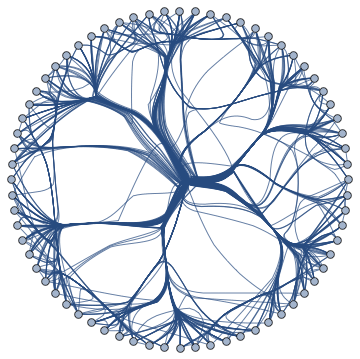
There are endless ways to manipulate and customize graphs in Mathematica. Here is an example of a hidden feature, the so-called edge bundling which bundles edges in order to achieve greater clarity.

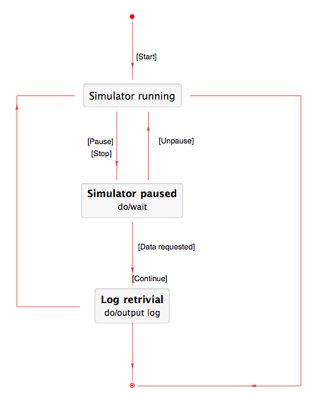
There are plenty of graph types in the software industry which are not directly available but which can be obtained with a bit of effort. Below is an example of a standard flowchart with the essential ingredient being the EdgeShapeFunction which we’ll discuss later on as well.

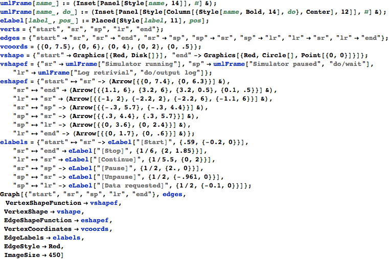
This results in a more traditional type of graph representation. While pretty much anything and everything is possible one should note though that Mathematica is more geared towards graph computations rather than graph representations.

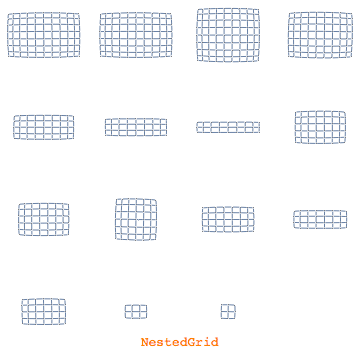
Mathematica is ideal for rapid prototyping of ideas and combining the multitude of functions. Here is an example of rectangular edges across different types of graph layouts

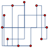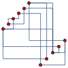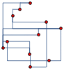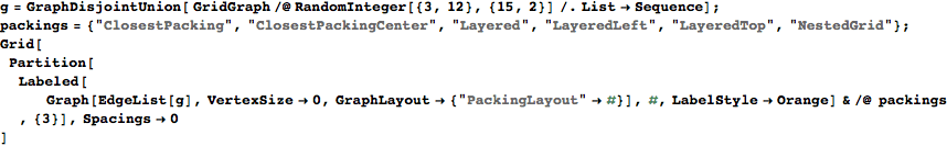
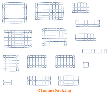
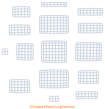
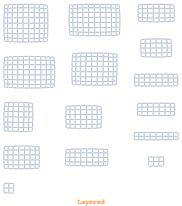
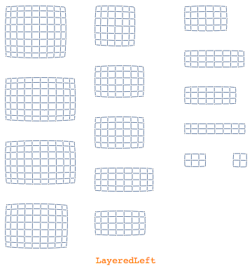
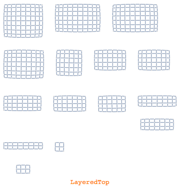
Graph layout is a world on its own and is closely related to graph analysis. Mathematica will by default automatically pick out the most appropriate layout for a given graph as well as the so-called graph packing. Graph packings are about how components of a graph are organized on top of the individual layout. Here is an overview of the possible component arrangements

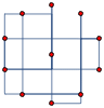
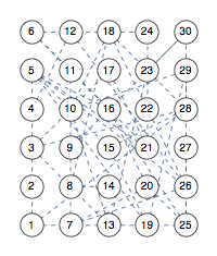
You can define your own layout of course and specify explicit coordinates. For example, here is an explicit grid layout

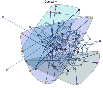
Elements of graphs can be highlighted as we showed above with London underground. Vertices belonging in some way together can also be visualized by means of the CommunityGraphPlot which in a way is a combination of graphs and sets.

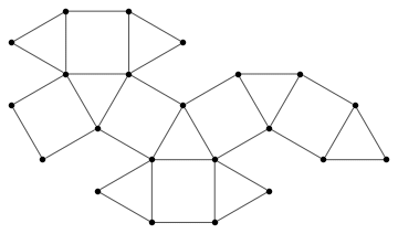
Yet another way to look at graphs is by considering the edges as segments of polygons.

Conversely, converting a checkered polygon to a graph is possible as well. Taking one of the polygons above we can convert it to a graphics of arrows

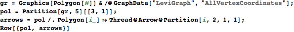
and take the coordinates which we then apply to a cycle graph;

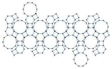
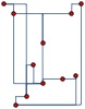
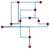
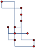
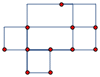
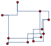
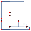
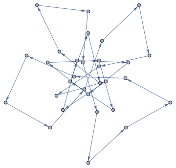
Floorplans and maze-like environment are really graphs and it’s easy to generate random mazes like so

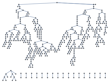
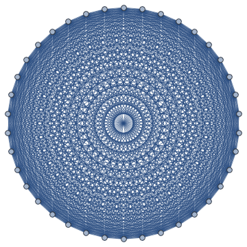
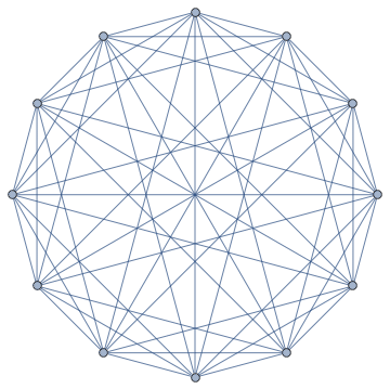
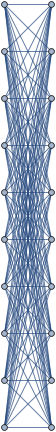
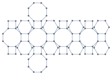
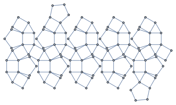
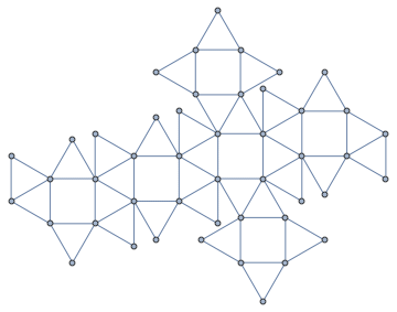
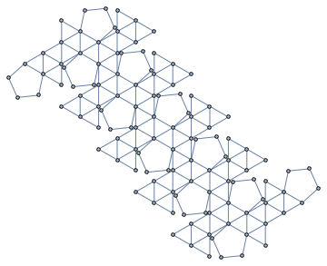
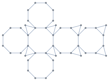
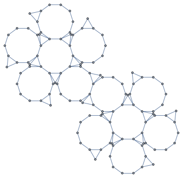
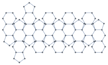
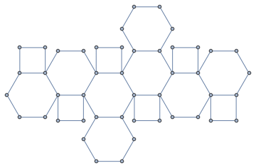
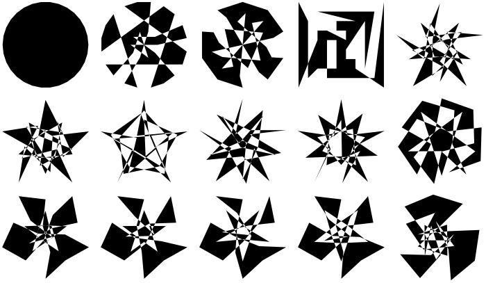
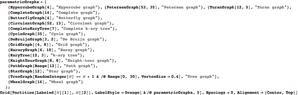
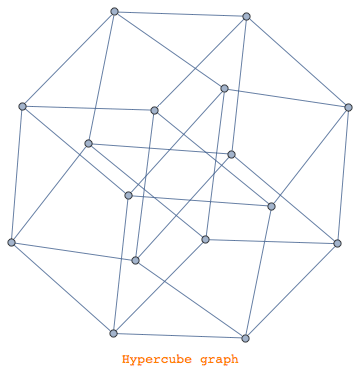
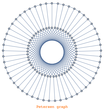
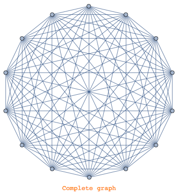
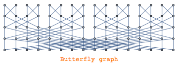
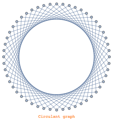
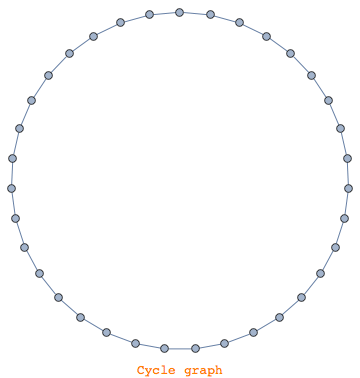
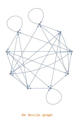
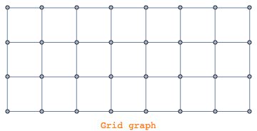
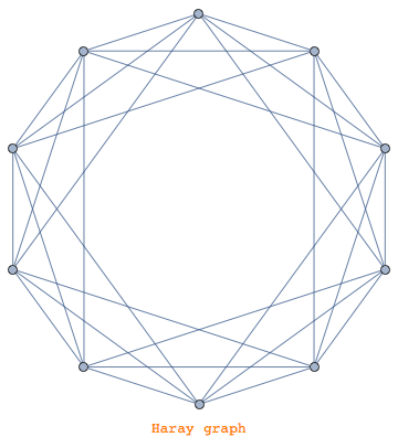
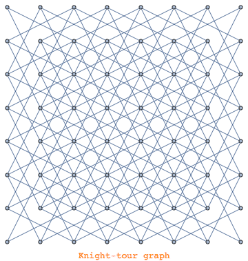
Mathematica contains a rich collection of so-called parametric graphs which have diverse types of regularities.

Besides all sorts of graphs with explicit names and the parametric graphs (like k-ary tree) there is a whole arsenal of ways to generate random graphs. There are many reasons why one would want to produce random graphs and it’s in fact an acadmic branch on its own. Among other:
– experiment with existing or invent new graph layout algorithms (graph embeddings)
– research collective behaviors or properties of graphs with certain constraints (statistical physics based on graphs)
– model epidemic and viral algorithms
– test out graph theoretic concepts (centrality and other measures)

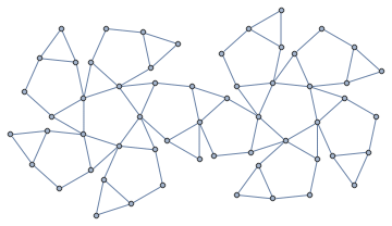
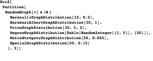
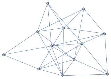
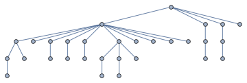
Here is a sample of random graphs based on various distributions:

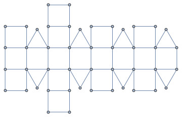
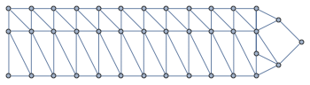
Sparse arrays are an important ingredient in graph drawing, most matrices deduced from a graph are sparse. Conversely, you can create graphs from sparse arrays. For example, the following ladder diagram is based on a banded sparse array

An interesting way to construct graphs is by looking at relationships between sets of objects. For example, the inclusion or subset operation gives a partially ordered set which can be made even more clear by looking at the so-called transitive reduction of the graph. The transitive reduction removes edges which can be deduced from the transitive closure.

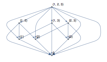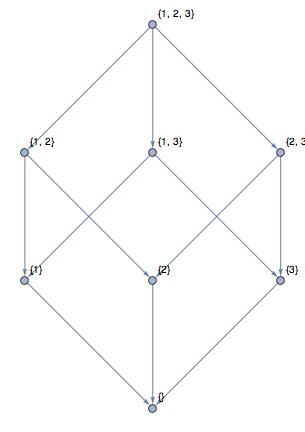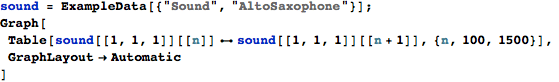
Finally, sound can also be converted to a graph by looking at the line graph outputted by default when loading a wave;

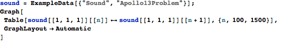
It produces beautiful floral patterns and is a good representation of the complexity of the data. For a comparison, here is the graph corresponding to the alt-sax