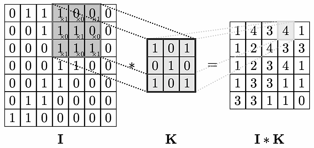
We can think of graphs as encoding a form of irregular spatial structure and graph convolutions attempt to generalize the convolutions applied to regular grid structures. Recall that if you have a grid like below you can glide a convolution matrix over it and the result at each step is the sum of the overlay (not a normal matrix multiplication!). If one looks at the grid as a graph then the convolution is simplified by the fact that one can use a global matrix across the whole graph. In a general graph this is not possible and one gets a location dependent convolution. This immediately infers that it takes more processing to perform a convolution on a graph than on, say, a 2D image.

This location dependence can however also vary in complexity. For example, if you have a central node with data $v_0$ surrounded by neighbors with data $v_i$ you could define a convolution so that the new data $v’_0$ at the node is
$$v’_0 = \sum \frac{1}{d_0\,d_i}v_i$$
with $d_i, d_0$ the vertex degrees. This is a nicely symmetric and easy to compute convolution. A more complex is the attention mechanism where one has an additional layer of complexity and parameters.

Enumerating the desirable traits of image convolutions, we arrive at the following properties we would ideally like our graph convolutional layer to have:

  • Computational and storage efficiency
  • Fixed number of parameters (independent of input graph size);
  • Localisation (acting on a local neighbourhood of a node);
  • Ability to specify arbitrary importances to different neighbours;
  • Applicability to inductive problems (arbitrary, unseen graph structures).
    Satisfying all of the above at once has proves to be challenging, and indeed, none of the prior techniques have been successful at achieving them simultaneously.

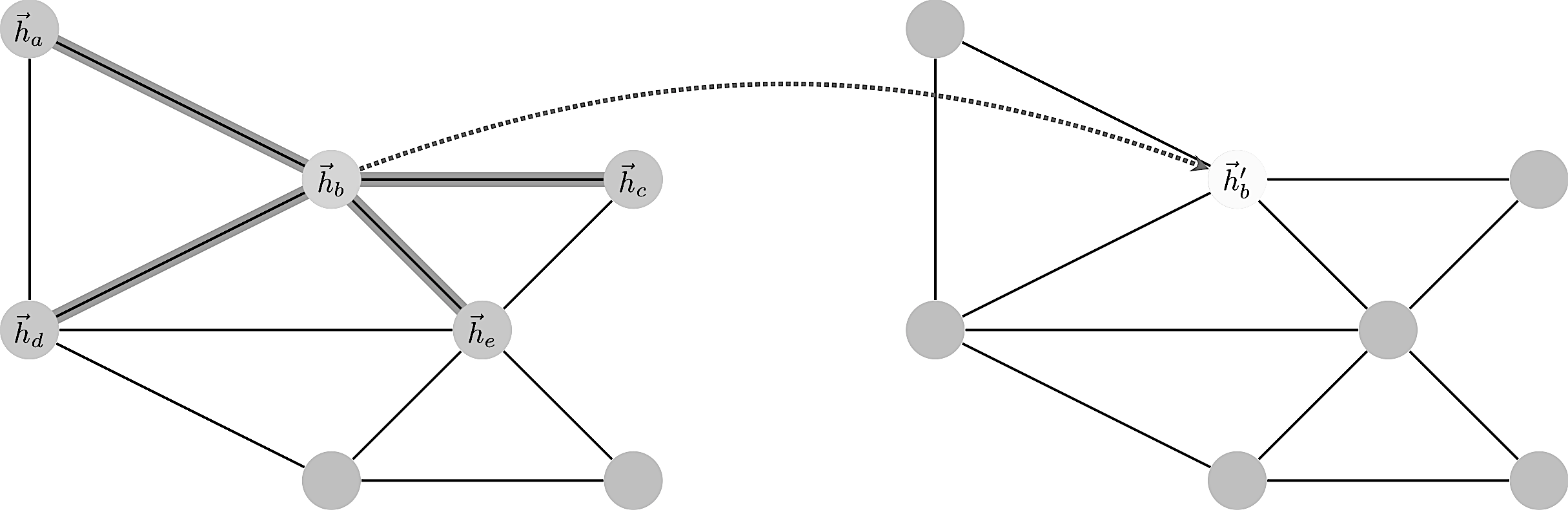
Consider a graph of $n$ nodes, specified as a set of node features $(f_1,\dots,f_n)$ and an adjacency matrix $(A_{ij})$. These two inputs completely define the graph as a structure we wish to work with.
A graph convolution computes a new set $(f’_1,\dots,f’_n)$ via a neural transformation
$$ \sigma ( \sum_{j\in n(i)}\alpha_{ij} f_j )$$
where the sum is over neighbors. The problem with this formula is to make the transformation independent of the local structure. How to define $\alpha$ such that it works in all contexts?
The trick is to let $\alpha_{ij}$ be implicitly defined, employing self-attention over the node features to do so. Self-attention has previously been shown to be self-sufficient for state-of-the-art-level results on machine translation, as demonstrated by the Transformer architecture
We let $\alpha_{ij}$ be computed as a byproduct of an attention mechanism which computes unnormalized coefficients $e_{ij}$ across pairs of nodes based on their features
$$e_{ij}=\alpha(f_i,f_j).$$
$$ f_i \mapsto \sigma(\sum_{j\in n(i)}\alpha(f_i,f_j)\;f_j)$$
Usually a softmax is applied over neighborhood to normalize things:
$$\alpha_{ij} = \frac{\exp(e_{ij})}{\sum_{n(i)}\exp(e_{ik})}$$
More details can be found in the original paper or this review paper.
In the following example we use once again the Cora dataset to show how GAT can be used to predict data on the nodes. In this case the ‘subject’ label of the paper represented by the node.

    import networkx as nx
    import pandas as pd
    import os
    import stellargraph as sg
    from stellargraph.mapper import FullBatchNodeGenerator
    from stellargraph.layer import GAT
    from keras import layers, optimizers, losses, metrics, Model
    from sklearn import preprocessing, feature_extraction, model_selection
Using TensorFlow backend.

See a related article for details about Cora, we simply reproduce a straightforward import to obtain a Stellargraph graph instance.

    data_dir = os.path.expanduser("~/data/cora")
    edgelist = pd.read_csv(os.path.join(data_dir, "cora.cites"), sep='\t', header=None, names=["target", "source"])
    edgelist["label"] = "cites"
    Gnx = nx.from_pandas_edgelist(edgelist, edge_attr="label")
    nx.set_node_attributes(Gnx, "paper", "label")
    feature_names = ["w_{}".format(ii) for ii in range(1433)]
    column_names =  feature_names + ["subject"]
    node_data = pd.read_csv(os.path.join(data_dir, "cora.content"), sep='\t', header=None, names=column_names)

For machine learning we want to take a subset of the nodes for training, and use the rest for validation and testing. We’ll use scikit-learn again to do this.
Here we’re taking 140 node labels for training, 500 for validation, and the rest for testing.

    train_data, test_data = model_selection.train_test_split(
        node_data, train_size=140, test_size=None, stratify=node_data['subject']
    )
    val_data, test_data = model_selection.train_test_split(
        test_data, train_size=500, test_size=None, stratify=test_data['subject']
    )

Note using stratified sampling gives the following counts:

    from collections import Counter
    Counter(train_data['subject'])
Counter({'Genetic_Algorithms': 22,
         'Neural_Networks': 42,
         'Theory': 18,
         'Reinforcement_Learning': 11,
         'Case_Based': 16,
         'Probabilistic_Methods': 22,
         'Rule_Learning': 9})

The training set has class imbalance that might need to be compensated, e.g., via using a weighted cross-entropy loss in model training, with class weights inversely proportional to class support. However, we will ignore the class imbalance in this example, for simplicity.
For our categorical target, we will use one-hot vectors that will be fed into a soft-max Keras layer during training:

    target_encoding = feature_extraction.DictVectorizer(sparse=False)
    train_targets = target_encoding.fit_transform(train_data[["subject"]].to_dict('records'))
    val_targets = target_encoding.transform(val_data[["subject"]].to_dict('records'))
    test_targets = target_encoding.transform(test_data[["subject"]].to_dict('records'))

We now do the same for the node attributes we want to use to predict the subject. These are the feature vectors that the Keras model will use as input. The CORA dataset contains attributes ‘w_x’ that correspond to words found in that publication. If a word occurs more than once in a publication the relevant attribute will be set to one, otherwise it will be zero.

    node_features = node_data[feature_names]
    train_targets[1:3]
array([[0., 0., 1., 0., 0., 0., 0.],
       [0., 0., 1., 0., 0., 0., 0.]])

Now create a StellarGraph object from the NetworkX graph and the node features and targets. It is StellarGraph objects that we use in this library to perform machine learning tasks on.

    G = sg.StellarGraph(Gnx, node_features=node_features)
    print(G.info())
StellarGraph: Undirected multigraph
 Nodes: 2708, Edges: 5278
 Node types:
  paper: [2708]
    Edge types: paper-cites->paper
 Edge types:
    paper-cites->paper: [5278]

To feed data from the graph to the Keras model we need a generator. Since GAT is a full-batch model, we use the FullBatchNodeGenerator class to feed node features and graph adjacency matrix to the model.

    generator = FullBatchNodeGenerator(G, method="gat")

For training we map only the training nodes returned from our splitter and the target values.

    train_gen = generator.flow(train_data.index, train_targets)

Now we can specify our machine learning model, we need a few more parameters for this:

  • the layer_sizes is a list of hidden feature sizes of each layer in the model. In this example we use two GAT layers with 8-dimensional hidden node features for the first layer and the 7 class classification output for the second layer.
  • attn_heads is the number of attention heads in all but the last GAT layer in the model
  • activations is a list of activations applied to each layer’s output
  • Arguments such as bias, in_dropout, attn_dropout are internal parameters of the model, execute ?GAT for details.
    gat = GAT(
        layer_sizes=[8, train_targets.shape[1]],
        activations=["elu", "softmax"],
        attn_heads=8,
        generator=generator,
        in_dropout=0.5,
        attn_dropout=0.5,
        normalize=None
    )
    

Expose the input and output tensors of the GAT model for node prediction, via GAT.node_model() method:

    x_inp, predictions = gat.node_model()
WARNING:tensorflow:From /Users/swa/conda/lib/python3.7/site-packages/tensorflow/python/ops/control_flow_ops.py:423: colocate_with (from tensorflow.python.framework.ops) is deprecated and will be removed in a future version.
Instructions for updating:
Colocations handled automatically by placer.
WARNING:tensorflow:From /Users/swa/conda/lib/python3.7/site-packages/keras/backend/tensorflow_backend.py:3445: calling dropout (from tensorflow.python.ops.nn_ops) with keep_prob is deprecated and will be removed in a future version.
Instructions for updating:
Please use `rate` instead of `keep_prob`. Rate should be set to `rate = 1 - keep_prob`.

Now let’s create the actual Keras model with the input tensors x_inp and output tensors being the predictions predictions from the final dense layer

    model = Model(inputs=x_inp, outputs=predictions)
    model.compile(
        optimizer=optimizers.Adam(lr=0.005),
        loss=losses.categorical_crossentropy,
        metrics=["acc"],
    )

Train the model, keeping track of its loss and accuracy on the training set, and its generalisation performance on the validation set (we need to create another generator over the validation data for this)

    val_gen = generator.flow(val_data.index, val_targets)

Create callbacks for early stopping (if validation accuracy stops improving) and best model checkpoint saving:

    from tensorflow.keras.callbacks import EarlyStopping, ModelCheckpoint
    if not os.path.isdir("logs"):
        os.makedirs("logs")
    es_callback = EarlyStopping(monitor="val_acc", patience=20)  # patience is the number of epochs to wait before early stopping in case of no further improvement
    mc_callback = ModelCheckpoint(
        "logs/best_model.h5",
        monitor="val_acc",
        save_best_only=True,
        save_weights_only=True,
    )

Train the model

    history = model.fit_generator(
        train_gen,
        epochs=50,
        validation_data=val_gen,
        verbose=2,
        shuffle=False,  # this should be False, since shuffling data means shuffling the whole graph
        callbacks=[es_callback, mc_callback],
    )
Epoch 1/50
 - 2s - loss: 2.0091 - acc: 0.1286 - val_loss: 1.8762 - val_acc: 0.3160
Epoch 2/50
 - 0s - loss: 1.8727 - acc: 0.2357 - val_loss: 1.7720 - val_acc: 0.3900
Epoch 3/50
 - 0s - loss: 1.7359 - acc: 0.3500 - val_loss: 1.6811 - val_acc: 0.3800
...
Epoch 47/50
 - 0s - loss: 0.4901 - acc: 0.8214 - val_loss: 0.5821 - val_acc: 0.8440
Epoch 48/50
 - 0s - loss: 0.4258 - acc: 0.8857 - val_loss: 0.5797 - val_acc: 0.8440
Epoch 49/50
 - 0s - loss: 0.4788 - acc: 0.8571 - val_loss: 0.5775 - val_acc: 0.8400
Epoch 50/50
 - 0s - loss: 0.4801 - acc: 0.8429 - val_loss: 0.5748 - val_acc: 0.8360

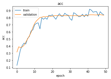
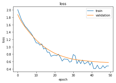
Plot the training history:

    import matplotlib.pyplot as plt
    %matplotlib inline
    def remove_prefix(text, prefix):
        return text[text.startswith(prefix) and len(prefix):]
    def plot_history(history):
        metrics = sorted(set([remove_prefix(m, "val_") for m in list(history.history.keys())]))
        for m in metrics:
            # summarize history for metric m
            plt.plot(history.history[m])
            plt.plot(history.history['val_' + m])
            plt.title(m)
            plt.ylabel(m)
            plt.xlabel('epoch')
            plt.legend(['train', 'validation'], loc='best')
            plt.show()
    plot_history(history)

png
png
Reload the saved weights of the best model found during the training (according to validation accuracy)

    model.load_weights("logs/best_model.h5")

Evaluate the best model on the test set

    test_gen = generator.flow(test_data.index, test_targets)
    test_metrics = model.evaluate_generator(test_gen)
    print("\nTest Set Metrics:")
    for name, val in zip(model.metrics_names, test_metrics):
        print("\t{}: {:0.4f}".format(name, val))
Test Set Metrics:
    loss: 0.6157
    acc: 0.8206

Now let’s get the predictions for all nodes:

    all_nodes = node_data.index
    all_gen = generator.flow(all_nodes)
    all_predictions = model.predict_generator(all_gen)

These predictions will be the output of the softmax layer, so to get final categories we’ll use the inverse_transform method of our target attribute specifcation to turn these values back to the original categories
Note that for full-batch methods the batch size is 1 and the predictions have shape $(1, N_{nodes}, N_{classes})$ so we we remove the batch dimension to obtain predictions of shape $(N_{nodes}, N_{classes})$.

    node_predictions = target_encoding.inverse_transform(all_predictions.squeeze())

Let’s have a look at a few predictions after training the model:

    results = pd.DataFrame(node_predictions, index=all_nodes).idxmax(axis=1)
    df = pd.DataFrame({"Predicted": results, "True": node_data['subject']})
    df.head(20)
Predicted True
31336 subject=Neural_Networks Neural_Networks
1061127 subject=Rule_Learning Rule_Learning
1106406 subject=Reinforcement_Learning Reinforcement_Learning
13195 subject=Reinforcement_Learning Reinforcement_Learning
37879 subject=Probabilistic_Methods Probabilistic_Methods
1126012 subject=Probabilistic_Methods Probabilistic_Methods
1107140 subject=Reinforcement_Learning Theory
1102850 subject=Neural_Networks Neural_Networks
31349 subject=Neural_Networks Neural_Networks
1106418 subject=Theory Theory
1123188 subject=Probabilistic_Methods Neural_Networks
1128990 subject=Neural_Networks Genetic_Algorithms
109323 subject=Probabilistic_Methods Probabilistic_Methods
217139 subject=Neural_Networks Case_Based
31353 subject=Neural_Networks Neural_Networks
32083 subject=Neural_Networks Neural_Networks
1126029 subject=Reinforcement_Learning Reinforcement_Learning
1118017 subject=Neural_Networks Neural_Networks
49482 subject=Neural_Networks Neural_Networks
753265 subject=Neural_Networks Neural_Networks

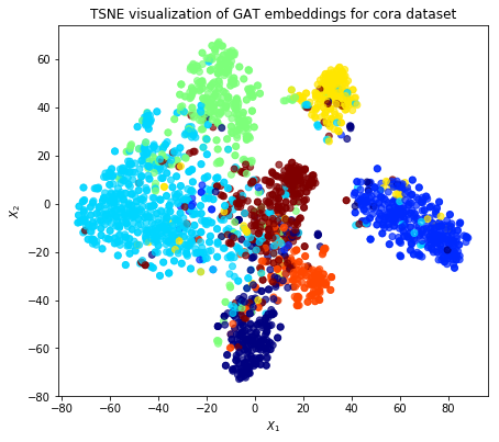
Evaluate node embeddings as activations of the output of the 1st GraphAttention layer in GAT layer stack (the one before the top classification layer predicting paper subjects), and visualise them, coloring nodes by their true subject label. We expect to see nice clusters of papers in the node embedding space, with papers of the same subject belonging to the same cluster.
Let’s create a new model with the same inputs as we used previously x_inp but now the output is the embeddings rather than the predicted class. We find the embedding layer by taking the first graph attention layer in the stack of Keras layers. Additionally note that the weights trained previously are kept in the new model.

    emb_layer = next(l for l in model.layers if l.name.startswith("graph_attention"))
    print("Embedding layer: {}, output shape {}".format(emb_layer.name, emb_layer.output_shape))
Embedding layer: graph_attention_sparse_1, output shape (1, 2708, 64)
    embedding_model = Model(inputs=x_inp, outputs=emb_layer.output)

The embeddings can now be calculated using the predict_generator function. Note that the embeddings returned are 64 dimensional features (8 dimensions for each of the 8 attention heads) for all nodes.

    emb = embedding_model.predict_generator(all_gen)
    emb.shape
(1, 2708, 64)

Project the embeddings to 2d using either TSNE or PCA transform, and visualise, coloring nodes by their true subject label

    from sklearn.decomposition import PCA
    from sklearn.manifold import TSNE
    import pandas as pd
    import numpy as np

Note that the embeddings from the GAT model have a batch dimension of 1 so we squeeze this to get a matrix of $N_{nodes} \times N_{emb}$.
Additionally, the GraphAttention layers before the final layer order the embeddings according to the graph order in G.nodes(), so we need to re-index the labels.

    X = emb.squeeze()
    y = np.argmax(target_encoding.transform(node_data.reindex(G.nodes())[["subject"]].to_dict('records')), axis=1)
    if X.shape[1] > 2:
        transform = TSNE #PCA
        trans = transform(n_components=2)
        emb_transformed = pd.DataFrame(trans.fit_transform(X), index=list(G.nodes()))
        emb_transformed['label'] = y
    else:
        emb_transformed = pd.DataFrame(X, index=list(G.nodes()))
        emb_transformed = emb_transformed.rename(columns = {'0':0, '1':1})
        emb_transformed['label'] = y
    alpha = 0.7
    fig, ax = plt.subplots(figsize=(7,7))
    ax.scatter(emb_transformed[0], emb_transformed[1], c=emb_transformed['label'].astype("category"),
                cmap="jet", alpha=alpha)
    ax.set(aspect="equal", xlabel="$X_1$", ylabel="$X_2$")
    plt.title('{} visualization of GAT embeddings for cora dataset'.format(transform.__name__))
    plt.show()

png

How to get started with the Cora dataset: import into a graph database, manipulate it and visualize it.

This notebook illustrates how Node2Vec can be applied to learn low dimensional node embeddings of an edge weighted graph through weighted biased random walks over the graph.
The example uses components from the stellargraph, Gensim, and scikit-learn libraries.
The following references can be useful:

Let’s import the necessary bits as usual. The most important one is Stellargraph:

    from sklearn.manifold import TSNE
    from sklearn.model_selection import train_test_split
    from sklearn.linear_model import LogisticRegressionCV
    from sklearn.metrics import accuracy_score
    from sklearn.metrics.pairwise import pairwise_distances
    from sklearn import preprocessing
    import os
    import networkx as nx
    import numpy as np
    import pandas as pd
    from stellargraph.data import BiasedRandomWalk
    from stellargraph import StellarGraph
    from gensim.models import Word2Vec
    import warnings
    import collections
    import matplotlib.pyplot as plt
    %matplotlib inline
Using TensorFlow backend.

The dataset is the citation Cora network. The Cora dataset consists of 2708 scientific publications classified into one of seven classes. The citation network consists of 5429 links. Each publication in the dataset is described by a 0/1-valued word vector indicating the absence/presence of the corresponding word from the dictionary. The dictionary consists of 1433 unique words. The README file in the dataset provides more details.
For this demo, we ignore the word vectors associated with each paper. We are only interested in the network structure and the subject attribute of each paper.
Download and unzip the cora.tgz file to a location on your computer, let’s assume it’s ~/data/cora/.

    data_dir = "~/data/cora"

Next, we create a normal undirected NetworkX graph:

    cora_location = os.path.expanduser(os.path.join(data_dir, "cora.cites"))
    g_nx_wt = nx.read_weighted_edgelist(path=cora_location, create_using=nx.DiGraph()).reverse()
    g_nx_wt = g_nx_wt.to_undirected()

Assign the ‘subject’ to the node:

    cora_data_location = os.path.expanduser(os.path.join(data_dir, "cora.content"))
    node_attr = pd.read_csv(cora_data_location, sep='\t', header=None)
    values = { str(row.tolist()[0]): row.tolist()[-1] for _, row in node_attr.iterrows()}
    nx.set_node_attributes(g_nx_wt, values, 'subject')

Select the largest connected component. For clarity we ignore isolated nodes and subgraphs; having these in the data does not prevent the algorithm from running and producing valid results.

    g_nx_wt = max(nx.connected_component_subgraphs(g_nx_wt, copy=True), key=len)
    print("Largest subgraph statistics: {} nodes, {} edges".format(
        g_nx_wt.number_of_nodes(), g_nx_wt.number_of_edges()))
Largest subgraph statistics: 2485 nodes, 5069 edges

For weighted biased random walks the underlying graph should have weights over the edges. Since the links in the Cora dataset are unweighted, we need to synthetically add weights to the links in the graph. One possibility is to weight each edge by the similarity of its end nodes. Here we assign the Jaccard similarity of the features of the pair of nodes as the weight of edge:

    df = node_attr.copy()
    df.set_index(0, inplace = True)
    papers = df.index
    ## calculating the paiwise jaccard similarity between each pair of nodes.
    with warnings.catch_warnings():
        warnings.simplefilter("ignore")
        wts = pd.DataFrame(
            1- pairwise_distances(df.iloc[:,:-1].values, metric = 'jaccard'),
            index = papers, columns = papers)
        wts.index = wts.index.map(str)
        wts.columns = wts.columns.map(str)

Append the weight attribute to the edges. Note, here we use the word ‘weight’ to label the weight value over the edge but it can be any other user specified label.

    for u,v in g_nx_wt.edges():
        val = wts[u][v]
        g_nx_wt[u][v]['weight'] = val

The weights distribution can be seen as follows:

    wts = list()
    for u,v in g_nx_wt.edges():
        wts.append(g_nx_wt[u][v]['weight'])
    wts = sorted(wts, reverse = True)
    edgeCount = collections.Counter(wts)
    wt, cnt = zip(*edgeCount.items())
    plt.figure(figsize=(10,8))
    plt.bar(wt, cnt, width=0.005, color='b')
    plt.title("Edge weights histogram")
    plt.ylabel("Count")
    plt.xlabel("edge weights")
    plt.xticks(np.linspace(0,1,10))
    plt.show()

png
The above distribution of edge weights illustrates that majority of linked nodes are insignificantly similar in terms of their attributes.
The Node2Vec algorithm is a method for learning continuous feature respresentations for nodes in networks. This approach can simply be described as a mapping of nodes to a low dimensional space of features that maximizes the likelihood of preservering neighborhood sgrtucture of the nodes. This approach is not tied to a fixed definition of neighborhood of a node but can be used in conjunction with different notions of node neighborhood, such as, homophily or structural equivalence, among other concepts. The algorithm efficiently explores diverse neighborhoods of nodes through a biased random walk procedure that is parametrized to emulate a specific concept of the neighborhood of a node.
Once a pre-defined number of walks, of fixed lengths, have been sampled, the low dimension embedding vectors of nodes can be learnt using Word2vec algorithm. We use the Word2Vec implementation in the Gensim library but any other can do.
The Stellargraph library provides an implementation of random walks that can be unweighted or weighted as required by Node2Vec. The random walks have a pre-defined fixed maximum length and are controlled by three parameters p, q, and weight. By default, the weight over the edges is assumed to be 1.
The first step for the weighted biased random walk is to build a random walk object by passing it a Stellargraph object.

    rw = BiasedRandomWalk(StellarGraph(g_nx_wt))

The next step is to sample a set of random walks of pre-defined length starting from each node of the graph. Parameters p, q, and weighted influence the type of random walks in the procedure. In this demo, we are going to start 10 random walks from each node in the graph with a length up to 100. We set parameter p to 0.5 and q to 2.0 and the weight parameter set to True. The run method in the random walk will check if the weights over the edges are available and resolve other issues, such as, whether the weights are numeric and that their is no ambiguity of edge traversal (i.e. each pair of node is connected by a unique numerically weighted edge).

    weighted_walks = rw.run(
        nodes=g_nx_wt.nodes(), # root nodes
        length=100,    # maximum length of a random walk
        n=10,          # number of random walks per root node
        p=0.5,         # Defines (unormalised) probability, 1/p, of returning to source node
        q=2.0,         # Defines (unormalised) probability, 1/q, for moving away from source node
        weighted=True, #for weighted random walks
        seed=42        # random seed fixed for reproducibility
    )
    print("Number of random walks: {}".format(len(weighted_walks)))
Number of random walks: 24850

Once we have a sample set of walks, we learn the low-dimensional embedding of nodes using Word2Vec approach.
We set the dimensionality of the learned embedding vectors to 128.

    weighted_model = Word2Vec(weighted_walks, size=128, window=5, min_count=0, sg=1, workers=1, iter=1)

To visualise node embeddings generated by weighted random walks we can use t-SNE.
We retrieve the Word2Vec node embeddings that are 128-dimensional vectors and then we project them down to 2 dimensions using the t-SNE algorithm for visualization.

    # Retrieve node embeddings and corresponding subjects
    node_ids = weighted_model.wv.index2word  # list of node IDs
    weighted_node_embeddings = weighted_model.wv.vectors  # numpy.ndarray of size number of nodes times embeddings dimensionality
    node_targets = [ g_nx_wt.node[node_id]['subject'] for node_id in node_ids]
    # Apply t-SNE transformation on node embeddings
    tsne = TSNE(n_components=2 , random_state=42)
    weighted_node_embeddings_2d = tsne.fit_transform(weighted_node_embeddings)

The values of weighted_node_embeddings_2d can be plotted:

    # draw the points
    alpha = 0.7
    label_map = {l: i for i, l in enumerate(np.unique(node_targets))}
    node_colours = [ label_map[target] for target in node_targets ]
    plt.figure(figsize=(10,8))
    plt.scatter(weighted_node_embeddings_2d[:,0],
                weighted_node_embeddings_2d[:,1],
                c=node_colours, cmap = "jet", alpha = 0.7)
    plt.show()

png
The node embeddings calculated using Word2Vec can be used as feature vectors in a downstream task such as node classification. Here we give an example of training a logistic regression classifier using the node embeddings, learnt above, as features.

    X = weighted_node_embeddings
    y = np.array(node_targets)

Note that you can mix embedding values and standard feature values in the full feature vector.
We use 75% of the data for training and the remaining 25% for testing as a hold out test set.

    X_train, X_test, y_train, y_test = train_test_split(
        X, y, train_size=0.75, test_size=None, random_state = 42
    )
    print("Array shapes:\n X_train = {}\n y_train = {}\n X_test = {}\n y_test = {}" \
          .format(X_train.shape, y_train.shape, X_test.shape, y_test.shape))
Array shapes:
 X_train = (1863, 128)
 y_train = (1863,)
 X_test = (622, 128)
 y_test = (622,)

A logistic regression is learned:

    clf = LogisticRegressionCV(
        Cs=10,
        cv=10,
        tol=0.001,
        max_iter=1000,
        scoring="accuracy",
        verbose=False,
        multi_class='ovr',
        random_state=5434
    )
    clf.fit(X_train, y_train)
LogisticRegressionCV(Cs=10, class_weight=None, cv=10, dual=False,
           fit_intercept=True, intercept_scaling=1.0, max_iter=1000,
           multi_class='ovr', n_jobs=None, penalty='l2', random_state=5434,
           refit=True, scoring='accuracy', solver='lbfgs', tol=0.001,
           verbose=False)

and, as always, we predict things to evaluate the accuracy of the model:

    y_pred = clf.predict(X_test)
    accuracy_score(y_test, y_pred)
0.8135048231511254

Comparison of weighted and unnweighted biased random walks

Lets compare weighted random walks with unweighted random walks. This simply requires toggling the weight parameter to False in the run method of the BiasedRandomWalk. Note, the weight parameter is by default set to False, hence, not specifying the weight parameter would result in the same action.

    walks = rw.run(
        nodes=g_nx_wt.nodes(), # root nodes
        length=100,     # maximum length of a random walk
        n=10,           # number of random walks per root node
        p=0.5,          # Defines (unormalised) probability, 1/p, of returning to source node
        q=2.0,          # Defines (unormalised) probability, 1/q, for moving away from source node
        weighted=False, # since we are interested in unweighted walks
        seed=42         # for reproducibility
    )
    print("Number of random walks: {}".format(len(walks)))
    model = Word2Vec(walks, size=128, window=5, min_count=0, sg=1, workers=1, iter=1)
Number of random walks: 24850

We use the same t-SNE trick to plot the embedding:

    # Retrieve node embeddings and corresponding subjects
    node_ids = model.wv.index2word  # list of node IDs
    node_embeddings = model.wv.vectors  # numpy.ndarray of size number of nodes times embeddings dimensionality
    node_targets = [ g_nx_wt.node[node_id]['subject'] for node_id in node_ids]
    # Apply t-SNE transformation on node embeddings
    tsne = TSNE(n_components=2, random_state=42)
    node_embeddings_2d = tsne.fit_transform(node_embeddings)
    # draw the points
    alpha = 0.7
    label_map = { l: i for i, l in enumerate(np.unique(node_targets))}
    node_colours = [ label_map[target] for target in node_targets]
    plt.figure(figsize=(10,8))
    plt.scatter(node_embeddings_2d[:,0],
                node_embeddings_2d[:,1],
                c=node_colours, cmap = "jet", alpha = 0.7)
    plt.show()

png
Visual comparison of node embedding plots for weighted and unweighted random walks illustrates the differences betweem the two.
Going a step further, we can see how the unweighted approach predicts things.

    # X will hold the 128-dimensional input features
    X = node_embeddings
    # y holds the corresponding target values
    y = np.array(node_targets)
    X_train, X_test, y_train, y_test = train_test_split(
        X, y, train_size=0.75, test_size=None, random_state=42
    )
    clf = LogisticRegressionCV(
        Cs=10,
        cv=10,
        tol=0.01,
        max_iter=1000,
        scoring="accuracy",
        verbose=False,
        multi_class='ovr',
        random_state=5434
    )
    clf.fit(X_train, y_train)
    y_pred = clf.predict(X_test)
    accuracy_score(y_test, y_pred)
0.8520900321543409

Generally, the node embeddings extracted from unweighted random walks are more representative of the underlying community structure of the Cora dataset than the embeddings learnt from weighted random walks over the artificially weighted Cora network.
Of course, this is not a general statement. Also note that we assigned weights in a particular synthetic fashion. If the weights are given the accuracy could be higher.

Testing whether weights = 1 gives identical result to unweighted randomwalks

Lastly, we demonstrate that weighted biased random walks are identical to unweighted biased random walks when weights over the edges are identically 1.
First, set weights of all edges in the graph to 1.

    for u,v in g_nx_wt.edges():
        g_nx_wt[u][v]['weight'] = 1

Quick check to confirm if all edge weights are actually 1.

    wts = list()
    for u,v in g_nx_wt.edges():
        wts.append(g_nx_wt[u][v]['weight'])
    wts = sorted(wts, reverse = True)
    edgeCount = collections.Counter(wts)
    wt, cnt = zip(*edgeCount.items())
    plt.figure(figsize=(10,8))
    plt.bar(wt, cnt, width=0.005, color='b')
    plt.title("Edge weights histogram")
    plt.ylabel("Count")
    plt.xlabel("edge weights")
    plt.xticks(np.linspace(0,1,10))
    plt.show()

png

    rw = BiasedRandomWalk(StellarGraph(g_nx_wt))
    weighted_walks = rw.run(
        nodes=g_nx_wt.nodes(), # root nodes
        length=100,    # maximum length of a random walk
        n=10,          # number of random walks per root node
        p=0.5,         # Defines (unormalised) probability, 1/p, of returning to source node
        q=2.0,         # Defines (unormalised) probability, 1/q, for moving away from source node
        weighted=True, # indicates the walks are weighted
        seed=42        # seed fixed for reproducibility
    )
    print("Number of random walks: {}".format(len(weighted_walks)))
Number of random walks: 24850

Compare unweighted walks with weighted walks when all weights are uniformly set to 1. Note, the two sets should be identical given all other parameters and random seeds are fixed.

    assert walks == weighted_walks
    weighted_model = Word2Vec(weighted_walks, size=128, window=5, min_count=0, sg=1, workers=1, iter=1)

If you once again plot the embedding you can see that unweighted and weight one embeddings are identical.

    # Retrieve node embeddings and corresponding subjects
    node_ids = weighted_model.wv.index2word  # list of node IDs
    weighted_node_embeddings = weighted_model.wv.vectors  # numpy.ndarray of size number of nodes times embeddings dimensionality
    node_targets = [ g_nx_wt.node[node_id]['subject'] for node_id in node_ids]
    # Apply t-SNE transformation on node embeddings
    tsne = TSNE(n_components=2, random_state=42)
    weighted_node_embeddings_2d = tsne.fit_transform(weighted_node_embeddings)
    # draw the points
    alpha = 0.7
    label_map = { l: i for i, l in enumerate(np.unique(node_targets))}
    node_colours = [ label_map[target] for target in node_targets]
    plt.figure(figsize=(10,8))
    plt.scatter(weighted_node_embeddings_2d[:,0],
                weighted_node_embeddings_2d[:,1],
                c=node_colours, cmap = "jet", alpha = 0.7)
    plt.show()

png
Compare classification of nodes through logistic regression on embeddings learnt from weighted (weight == 1) walks to that of unweighted walks demonstrated above.

    # X will hold the 128-dimensional input features
    X = weighted_node_embeddings
    # y holds the corresponding target values
    y = np.array(node_targets)
    X_train, X_test, y_train, y_test = train_test_split(
        X, y, train_size=0.75, test_size=None, random_state=42
    )
    print("Array shapes:\n X_train = {}\n y_train = {}\n X_test = {}\n y_test = {}" \
          .format(X_train.shape, y_train.shape, X_test.shape, y_test.shape))
Array shapes:
 X_train = (1863, 128)
 y_train = (1863,)
 X_test = (622, 128)
 y_test = (622,)
    clf = LogisticRegressionCV(
        Cs=10,
        cv=10,
        tol=0.001,
        max_iter=1000,
        scoring="accuracy",
        verbose=False,
        multi_class='ovr',
        random_state=5434
    )
    clf.fit(X_train, y_train)
    y_pred = clf.predict(X_test)
    accuracy_score(y_test, y_pred)
    np.array_equal(weighted_node_embeddings, node_embeddings)
True

The weighted random walks with weight == 1 are identical to unweighted random walks. Moreover, the embeddings learnt over the two kinds of walks are identical as well.

Embedding of nodes happens via word2vec by means of a smart trick: using randomg walks over the graph to generate ‘word’ sequences.
Stellargraph has its own direct method to perform the embedding but the intermediate methods highlights better the process. So, below we generate the node2vec embedding via an explicit walk and show how it generates a really good community detection separation.

    import networkx as nx
    import numpy as np
    import matplotlib.pyplot as plt
    from sklearn.manifold import TSNE
    %matplotlib inline

We’ll use the karater club to demonstrate the process. The graph consists of two sets of nodes which are a well-separated according to the ‘club’ property.

    g_nx = nx.karate_club_graph()
    cols = ["green" if g_nx.nodes[n]["club"]=='Officer' else "orange" for n in g_nx.nodes()]
    nx.draw(g_nx, node_color=cols)

png
From this graph we create a Stellargraph and perform a biased random walk on it. This generates word sequences, in this case the string value of the node index.

    from stellargraph.data import BiasedRandomWalk
    from stellargraph import StellarGraph
    from gensim.models import Word2Vec
    rw = BiasedRandomWalk(StellarGraph(g_nx))
    walks = rw.run(
          nodes=list(g_nx.nodes()), # root nodes
          length=100,  # maximum length of a random walk
          n=10,        # number of random walks per root node
          p=0.5,       # Defines (unormalised) probability, 1/p, of returning to source node
          q=2.0        # Defines (unormalised) probability, 1/q, for moving away from source node
    )
    walks = [list(map(str, walk)) for walk in walks]
    model = Word2Vec(walks, size=128, window=5, min_count=0, sg=1, workers=2, iter=1)

The value of an embedding is for instance

    model.wv['29']
array([ 0.0283457 ,  0.06906749, -0.09740856,  0.08761664,  0.0240158 ,
       -0.04252268,  0.05366189,  0.12255755, -0.14192946, -0.12441556,
        0.14022443,  0.16821992,  0.01899681,  0.02525605, -0.129657  ,
       -0.00075872, -0.10963597, -0.24603637,  0.14481993,  0.04069758,
       ...
       -0.03686432,  0.28888953,  0.06754036], dtype=float32)

In order to visualize the embedding one has to somehow reduce the dimension. This is most easily done via t-SNE.

    # Retrieve node embeddings and corresponding subjects
    node_ids = model.wv.index2word  # list of node IDs
    node_embeddings = model.wv.vectors  # numpy.ndarray of size number of nodes times embeddings dimensionality
    node_targets = [ g_nx.node[int(node_id)]['club'] for node_id in node_ids]
    # Apply t-SNE transformation on node embeddings
    tsne = TSNE(n_components=2)
    node_embeddings_2d = tsne.fit_transform(node_embeddings)
    alpha=0.9
    label_map = { l: i for i, l in enumerate(np.unique(node_targets))}
    node_colours = [ label_map[target] for target in node_targets]
    plt.figure(figsize=(10,8))
    plt.scatter(node_embeddings_2d[:,0],
                node_embeddings_2d[:,1],
                c=node_colours, cmap="jet", alpha=alpha)
<matplotlib.collections.PathCollection at 0x1463cfc50>

png
This looks like a clean separation indeed. The splitting is not 100% correct though, just by looking at the corresponding value of the ‘club’ property.

    [g_nx.nodes[i] for i,v in enumerate(node_colours) if v==1]
[{'club': 'Mr. Hi'},
 {'club': 'Mr. Hi'},
 {'club': 'Mr. Hi'},
 {'club': 'Officer'},
 {'club': 'Mr. Hi'},
 {'club': 'Officer'},
 {'club': 'Officer'},
 {'club': 'Officer'},
 {'club': 'Mr. Hi'},
 {'club': 'Officer'},
 {'club': 'Officer'},
 {'club': 'Officer'},
 {'club': 'Officer'},
 {'club': 'Officer'},
 {'club': 'Officer'},
 {'club': 'Officer'},
 {'club': 'Officer'}]

Five out of senteen are incorrect. This is still remarkable considering the fact that node2vec process did not know anything at about the ‘club’ property but that it’s an emergent feature of the embedding.