In the past twenty years we have served and helped customers in many ways, all centered around graphs and how to enable a particular business vision with the help of graphs. There is usually the need for graph visualization and reporting in some way and this leads to the development of (custom) dashboard-like solutions. The challenge is always the fact that when it comes to reporting all solutions (say, PowerBI, Tableau and alike) are for relational data and not graph databases. For good reasons, the tabular format is easier to ‘linearize’ into a pie chart or a data grid.

In the same way, whenever you have graphs there is the need to edit them, the standard CRUD (create, read, update, delete) challenge. Here as well, there are tons of solutions for SQL backends but few for graphs. The OGMs (object graph models) are usually for Neo4j.

The re-creation of the same thing over and over again (as a consultant delivering bespoke solutions) is related to the fact that the intellectual property has to be unique and that in principle one can reuse some bits of code, in theory it never is that easy. Frameworks change, different backend flavors, different technologies. The technology landscape is every day a new challenge.

So, despite all constraints and challenges we set out to develop something best described as a stepping stone for graph-driven applications. The result is called Qwiery and is a set of open source tools to develop apps on top of graph stores.

Qwiery contains things like:

  • a flexible data access layer
  • a set of components to develop dashboards, terminals, notebook interfaces
  • wrappers around our favorite graph visualization frameworks (yFiles, Ogma, Cytoscape…)
  • utilities (working with datetime, strings, durations, colors…)
  • entities and messages
  • graphs (trees, graphs, random graphs, traversals…)

and much more. Each of these elements deserve a blog post on its own and the extensible data access layer is, in particular, a world on its own.

As show-cases we developed two full-fledge apps using Qwiery: Qwiery Dashboards and Qwiery Editor.

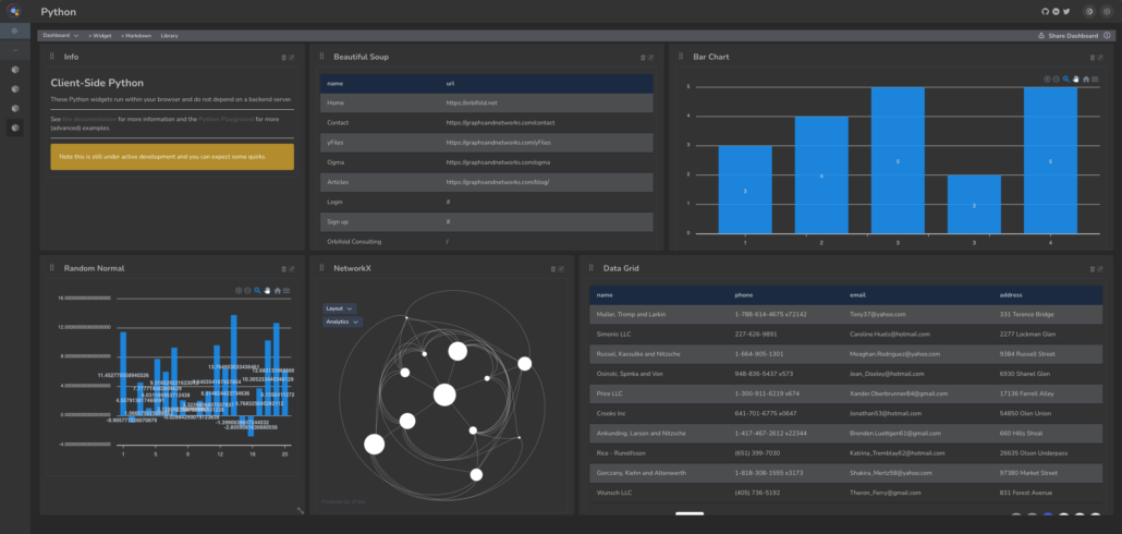
Qwiery Dashboards is a dashboarding app for graphs. It comes with:

  • widgets specifically designed to query Cypher (property graph) databases like Neo4j and MemGraph
  • client-side Python integration (enabling NetworkX, scikit-learn, pandas and numpy within the dashboards)
  • yFiles graph visualization
  • datagrids, pie chart, bar chart and all that

You can see the app deployed here.

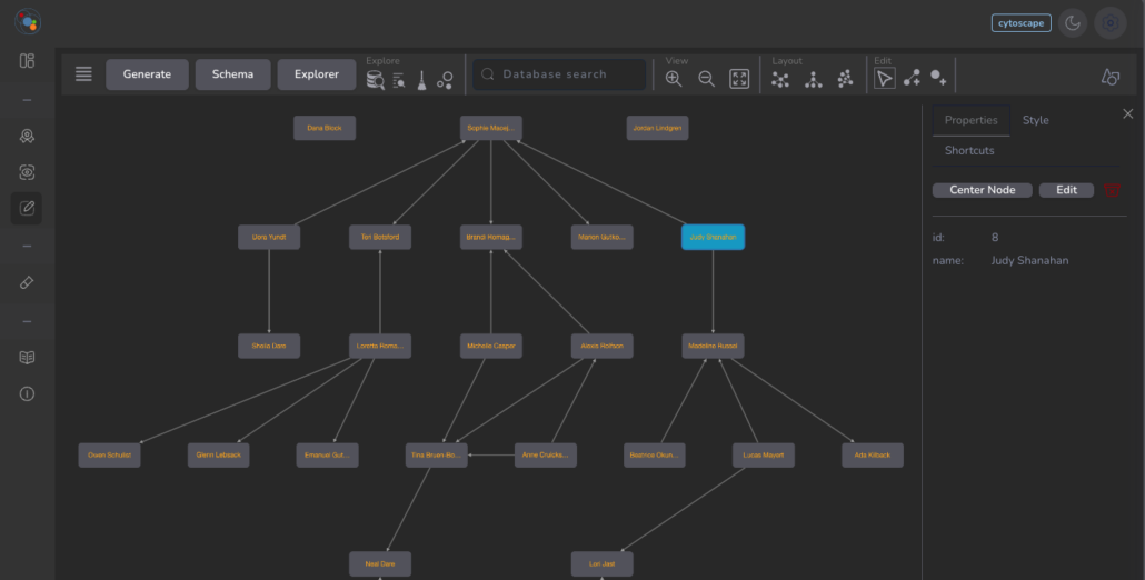
Qwiery Editor is a fairly standard graph editing app with:

  • a pluggable graph visualization component (you can use yFiles or Ogma if you own a license, otherwise the Cytoscape wrapper will do as well)
  • a Bloom clone of the path-query (that is, you can fetch data using a visual selector instead of writing Cypher)
  • the usual CRUD functionality you can also find in tools like Graphlytic and similar

Most of the elements are open source under the MIT license and available on GitHub, and/or via NPM packages.

In addition, we have backend services (in Python, NodeJs and .Net) allowing to go beyond the open source offering and giving a lot more juice. Please contact us for more information.

Companies transitioning to or adopting Neo4j inevitably face the challenge of getting large amounts of (legacy) data into their new (knowledge) graph. This often entails a large discussion about how to organize things (aka the ontology or graph schema) and how to technically make it happen. The ontological aspect is on its own quite an important topic but this article focuses on the technical effort.

When ingesting large amounts of data (tens of Gb) into Neo4j there really is only one option: the neo4j-admin import utility. Everything else, including the ‘Load CSV‘ Cypher path is too slow to consider. The CLI import utility does the job but it also erases all existing data and you need a few post-fixes (restarting the database e.g.). Once the baseline is set the incremental data changes are usually discussed in the context of a CDC solution (change data capture) and this is where the non-destructive (Cypher-Bolt based) ingestion options come in. Companies often use cloud solutions (e.g. AWS Kinesis) or Apache Kafka for streaming data changes while static or almost static data changes require some form of scheduler and workflow platforms. This is where I advise customers to consider Apache Airflow, Apache Hop or messaging systems like RabbitMQ and alike.

Apache Airflow is a Python platform and this is also one of the main selling points for companies with a focus on data science (and/or a strong Python stack). Something like Apache Hop is an alternative but the typical Java context is often more difficult to digest for Python developers. Many customers like AWS Glue and other data platforms available on AWS or Azure, but the main disadvantage is the fact that these ETL platforms focus on marshaling relational or tabular data. Neo4j or similar graph backends are not very much supported by AWS Glue. So, when it comes to Neo4j ETL on premise or in the cloud (or both), Airflow is an ideal solution and one I like to advertise when companies request an ETL, CDC or inception solution.

The remains of this article describes the typical customer scenario:

  • how to get tons of data into a brand new Neo4j database
  • how to update the graph on regular intervals or explicitly when necessary
  • how to approach Airflow development to create a robust ETL solution.

The focus here is on how to ingest data in Neo4j but the blueprint below really works with any data source and any endpoint. Airflow is capable of marshaling between lots of things, it’s very much a plumbing toolbox.

Before diving into the technicalities, a few words and thoughts on the good and the lesser of Airflow. Like all of the Apache tools and frameworks, Airflow has its quirks and open source challenges. It’s not polished and it comes with a learning curve. Many Apache frameworks (say Apache Hop or Apache Hadoop) are Java based and the fact that Airflow is fully Python helps a lot in understanding things, since one can peek at the implementation. The terminology is not very standard and other things can lead one astray. For example, a task is not an element of a flow but rather the flow itself while the term ‘operator’ is used for flow steps. The term DAG (direct acyclic graph) is used to refer to a flow. I think it would help a lot if Airflow would rephrase a few things.

On a UI level things are also rather mediocre, but that’s almost a trademark of Apache. The thing that remains rather incomprehensible is why one can’t upload/update a flow via the UI. Meaning that in order to manage/add flows one needs access to the underlying OS (directories). This, in a way, indicates how to develop things with/for Airflow: you need to develop things locally and hand it over to some admin once it’s ready. Airflow can’t really be used as a service backend. If there is a DAG set up it can be managed and the UI is effective but it fails miserably towards development purposes.

On the upside, Airflow can be used for anything and everything you wish to schedule. It can connect to anything and if you can program it in Python you can run it in Airflow. This includes things like reaching out to AWS SageMaker, triggering workflows based on directory changes (so-called sensors), ingesting any type of data and so on.

Airflow is NOT designed for streaming data, that’s where Apache Kafka comes in. Airflow data needs to be static. You can schedule things as often as you like but Airflow does not run hot.

Airflow does not replace some due diligence. To be specific, Airflow will run flows which can last days but it’s not a solution for poorly written code and poor performance. You need to research the various servers and services before trying to connect them. With respect to Neo4j, the classic Cypher loading approach takes days if you have tens of Gb but takes minutes via the import utility.

The main development challenge when creating an Airflow DAG is how to run and debug it:

  • the essential thing to understand is that the flows in Airflow are scripts in a directory. By giving multiple people access to this you easily end up with clashing pip dependencies and custom functions.
  • if you execute a DAG via the UI you will see log output but the cycle of copy-pasting new code in a directory, running the DAG and looking at the log is obviously not productive. It also means you have access to the DAG directory of Airflow.
  • Airflow does not enforce a particular code organization and without it the management of flows can easily get out of hand

Towards a production-level ETL platform one needs:

  • DAG templates, in order to have a uniform directory strucuture which can be managed and understood
  • local development and unit tests prior to Airflow deployment
  • CI/CD pipelines from Github (or alike) which take over the DAG, set up the (environment) variables, pip dependencies, connections and so on.

The inclusion of contextual elements (vars, connections….) is something the Astronomer solution does well and is unfortunately not part of Airflow. The crux here is that every flow depends on some settings which can (and should) be defined on the Airflow level (see below). Setting up a DAG hence means also setting up these variables which either are well-defined in some documentation or need to be communicated. It would be easier to have a protocol in place as part of the DAG template which defines what the variables are and what value they need.

A separate dashboard of the DAG outputs would be also a great thing to have but this demands some custom web development (accessing the Airflow Rest API).

Local setup

There are various ways you can set up Apache Airflow locally:

The standard Conda setup is the preferred way to go because it allows easier setup of packages, access to configuration and, well, full control in general:

  • create a normal conda env, something like conda create --name airflow python=3.9
  • install airflow in it
  • initial a database (airflow db init)

The lightweight database solution out of the box is Sqlite but it’s advized to set up Postgresql.

Once this is set up you have a dag-directory wherein you can dump flows. The easiest way to test them is via

airflow dags test your-dag

which runs the flow in the same way as you would trigger it via the UI but it does not leave a log trace in the database. This does allow one to debug things with breakpoints and all that. If you want to debug things that way you need to refactor your Python code and debug/unit-test things like any other Python script.

Neo4j provider

Airflow has a Neo4j provider but it’s a lightweight implementation lacking the necessary bits to create an ETL flow. The ETL developed below uses the standard Bolt Neo4j driver and it needs to be installed with

pip install neo4j

Overview of an Airflow ETL

As mentioned above, loading several Gb of CSV data into Neo4j via the standard Cypher (either Create or Load CSV) path takes days. This approach works well for incremental changes and near realtime changes. The only fast and efficient way to load a large amount of data is via the neo4j-admin utility. It means, however, that

  • it erases any existing data
  • you need access/permission to the executable
  • you need to restart the Neo4j database (and often explicitly restart it via Cypher as well).

So, although this batch import has been developed for Airflow, it still requires a manual post-fix.

The various operators (DAG steps) are on their own useful for similar jobs and the whole flow is demonstrative of how things should be organized in general.

The starting point is a PyArrow Feather file. It takes just a couple of lines to convert a CSV to a Feather file and it decreases the file size tremendously. You can use Parquet or even the original CSV but it’s clear that CSV is a wasteful format.

The ETL can either load data via the aformentioned LOAD CSV way or via the neo4j-admin (batch) utility. This decision is made on the basis of the configuration.

# ============================================================
# ETL of sone raw data.
# - topn: take only the specified amount of the data source (default: -1)
# - transform: whether to transform the raw data or use the (supposedly present) clean feather file
# - import: can be 'none', 'batch' or 'load' (default: 'load'). The batch means that the batch CSV format is created for use with the neo4j-admin import CLI. The load means the Cypher LOAD CSV will be used.
#
# The following variables are expected:
#
# - data_dir: where the source data is
# - working_dir: a temporary directory
# - neo4j_db_dir: the root directory of the Neo4j database
# ============================================================
@dag(
    schedule="@once",
    start_date=datetime(2023, 1, 1),
    catchup=False,
    default_args={
        "retries": 1
    },
    dag_id="KG_ETL",
    description="Imports the the raw csv.",
    params={
        "topn": -1,
        "transform": True,
        "import": "batch",
        "cleanup": False
    },
    tags=['Xpertise'])

The default configuration can be overriden when testing like so

airflow dags test kg_etl --config="{'import':'load'}"

The configuration helps to run part of the flow. For example, if you want to only transform part of the raw data to the necessary CSV files (nodes and edges) you can use

airflow dags test kg_etl --config="{'topn':1000, 'transform':true, 'import':'none'}"

This takes the first 1000 rows and creates nodes.csv and edges.csv without importing anything in Neo4j.

The reading and transformation phases are standard Pandas operations and data wrangling. Neo4j needs in all cases the three CSV files for import and they have to sit in the import directory of the database. So, this database directory is necessarily a parameter of the DAG. The extra step necessary is to copy/move the generated files to this directory. This bash operation is either a simple cp or ssh (scp) command depending the topology of the solution.

Once the files are in the database directory they can be loaded in one of the two ways (batch or load). This is where either a Bolt connection is set up or where the neo4j-admin utility is called.

Directories

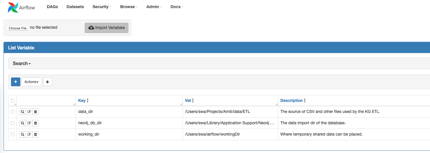
The following directories have to be configured on Airflow

  • datadir: the source of data (CSV or Feather file)
  • workingdir: a temporary directory
  • neo4jdbdir: the root of the database. This directory contains underneath the bin/neo4j-admin and the import directory. Neo4j will not import from anywhere else but this directory, unfortunately. It is possible to use http:// rather than file:// but with very large files this is not practical.

Directory structure

The organization can be used as a template for all Airflow efforts:

  • operators Contains the DAG operators
  • shared Contains the shared Python functions, constants and alike
  • main.py The main DAG
  • requirements.txt The Python package dependencies in a classic pip format
  • variables.json The variables which have to be defined in Airflow
  • connections.json The connections which have to be defined in Airflow.

The requirements, variables and connections should be used by a CI/CD pipeline to set things during deployment to Airflow.

Main DAG

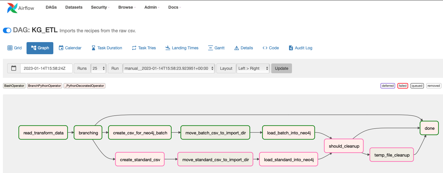
The way one defines a flow (see the diagram above) in Airflow is somewhat idiosyncratic. The main file contains the necessary preambles as well as the flow definition:

@dag(
    schedule="@once",
    start_date=datetime(2023, 1, 1),
    catchup=False,
    default_args={
        "retries": 1
    },
    dag_id="KG_ETL",
    description="Imports the graph from the raw csv.",
    params={
        "topn": -1,
        "transform": True,
        "import": "batch",
        "cleanup": False
    },
    tags=['Xpertise'])
def flow():
    etl = read_transform_data()
    what = which_import
    load_standard = load_standard_into_neo4j()
    load_batch = load_batch_into_neo4j()
    move_standard_csv = move_standard_csv_to_import_dir
    move_batch_csv = move_batch_csv_to_import_dir
    standard_csv = create_standard_csv()
    batch_csv = create_csv_for_neo4j_batch()
    clean_up_decision = should_cleanup
    end = done()

    etl >> what

    what >> standard_csv >> move_standard_csv >> load_standard
    what >> batch_csv >> move_batch_csv >> load_batch
    load_standard >> clean_up_decision
    load_batch >> clean_up_decision
    clean_up_decision >> temp_file_cleanup
    temp_file_cleanup >> end
    clean_up_decision >> end
    what >> end

flow = flow()

The names used in this flow definition are one-to-one with the operators defined. These operators are in essence just Python function and bash commands but do consult the docs for the many operator you can engage in a flow.

Variables

The variables.json defines the variables which have to be set in Airflow. The format is straightforward and needs to be used by CI/CD during deployment.

{
    "data_dir": {
        "value": "/Users/me/Projects/ETL",
        "description": "The source of CSV and other files used by the KG ETL."
    },
    "neo4j_db_dir": {
        "value": "/Users/me/Library/Application Support/Neo4j Desktop/Application/relate-data/dbmss/dbms-b8ef492f-0c84-4b56-8d83-a6d4f3b800e0",
        "description": "The data import dir of the database."
    },
    "working_dir": {
        "value": "/Users/me/temp",
        "description": "Where temporary shared data can be placed.",
    }
}

These variables are accessed in a flow like this:

working_dir = Variable.get_variable_from_secrets("working_dir")

Connections

Just like variables, a connection is a setting defined in Airflow which can be accessed inside the operators.

The ETL uses only the knowledge-graph connection to Neo4j:

{
    "knowledge-graph": {
        "id": "knowledge-graph",
        "host": "super-secret.neo4j.io",
        "schema": "neo4j+s",
        "login": "neo4j",
        "password": "neo4j",
        "port": 7687,
        "type": "neo4j"
    }
}

and it can be accessed like so in the DAG:

def get_connection():    
        con = Connection.get_connection_from_secrets("knowledge-graph")
        print( f"{con.schema}://{con.host}:{con.port}")

Requirements

The requirements files is like any Python project a set of packages:

neo4j
pandas
numpy
...

It should be used in a CI/CD pipeline to set up the Python environment.

This automatically brings up the issue of clashing packages for different flows. The way this can be resolved is via the @task.virtualenv attribute, for example

@task.virtualenv(
        task_id="virtualenv_python", requirements=["colorama==0.4.0"], system_site_packages=False
    )
    def callable_virtualenv():
        """
        Example function that will be performed in a virtual environment.

        Importing at the module level ensures that it will not attempt to import the
        library before it is installed.
        """
        from time import sleep

        from colorama import Back, Fore, Style

        print(Fore.RED + "some red text")
        print(Back.GREEN + "and with a green background")
        print(Style.DIM + "and in dim text")
        print(Style.RESET_ALL)
        for _ in range(4):
            print(Style.DIM + "Please wait...", flush=True)
            sleep(1)
        print("Finished")

    virtualenv_task = callable_virtualenv()

In addition, one can also use the following operators to have a clean separation:

  • PythonVirtualeEnvOperator – this one will build new virtualenv every time it needs one so might be a little brittle
  • KubernetesPodOperator – where you can have different variant of the images with different environments and choose the one you want for each task (requires Kubernetes)
  • DockerOperator – same as KubernetesPodOperator, but requires just Docker engine

Of course, there is also the option to access lambda function and whatnot in the cloud.

ETL Operators

There are some complex things in Airflow but this example is to show that things can be also quite easy. The DAG step to move files from one place to another looks like this:

# this is the source data
data_dir = Variable.get_variable_from_secrets("data_dir")
# this is the temp data
working_dir = Variable.get_variable_from_secrets("working_dir")
# the dir of the Neo4j database
neo4j_db_dir = Variable.get_variable_from_secrets("neo4j_db_dir")
neo4j_import_dir = os.path.join(neo4j_db_dir, "import")

move_standard_csv_to_import_dir = BashOperator(
    task_id="move_standard_csv_to_import_dir",
    bash_command= f"""
    mv '{os.path.join(working_dir,node.csv)}' '{neo4j_import_dir}' && mv '{os.path.join(working_dir, edges.csv)}' '{neo4j_import_dir}'
    """
    )

Batch loading of the CSV files is also quite simple

@task()
def load_batch_into_neo4j(**ctx):
    cmd = BashOperator(
        task_id='csv_batch_load',
        bash_command='bin/neo4j-admin database import full --delimiter="," --multiline-fields=true --overwrite-destination --nodes=import/nodes.csv --relationships=import/edges.csv  neo4j',
        cwd=neo4j_db_dir
    )

    cmd.execute(dict())
    say("Batch load done. Please restart the db in order to have the db digest the import.")
    # possibly requires a 'start database neo4j' as well

The tricky part resides in the correct parametrization and orchestration of tasks like these.

The actual data wrangling is really unrelated to Airflow is like any other Pandas effort. You can do all the hard work in Jupyter and paste the result in a task, for example:

@task()
def create_standard_csv(**ctx):
    """
        Creates the CSV files for LOAD CSV via cypher.
    """
    ti = ctx["ti"]
    params = ctx["params"]

    # ============================================================
    # Load data
    # ============================================================
    clean_feather_file = ti.xcom_pull(
        key='clean_feather_file', task_ids='read_transform_data')
    if clean_feather_file is None:
        raise Exception("Failed to get the clean_feather_file path.")
    if not os.path.exists(clean_feather_file):
        raise Exception(f"Specified file '{clean_feather_file}' does not exist.")

    df = pd.read_feather(clean_feather_file)
    logging.info("Found and loaded clean data")

    # ============================================================
    # Nodes
    # ============================================================
    nodes_file = create_nodes_csv(df, False, True)

    ti.xcom_push("nodes_csv_file", nodes_file)
    logging.info(f"Nodes CSV saved to '{nodes_file}'")

The create_nodes_csv call is where you can paste your Jupyter wrangling code. The XCOM push and pull methods is Airflow’s way to exchange (small amounts of) data between tasks. Here again, I think that the terminology is awkward, it obfuscates adoption and understanding.

Closing thoughts

All of the Apache frameworks and tools have the same mixture of good-bad (or love-hate if you prefer) and it always takes some time and energy to learn the ins and outs. Airflow is a stable ETL platform and if Python is your programming language it’s a great open source solution. Like any OSS it requires learning and additional embedding efforts.

Personally, I very much enjoy working with Airflow and would recommend it to any customer in need of an ETL solution and a Neo4j CDC or data ingestion need in particular.

Memgraph is a very promising product and I sincerely hope it will mature in the coming years to become an enterprise-ready alternative to Neo4j. I must admit, I really like it. It’s not battle-ready and much in flux but if the Memgraph guys manage to elevate it, it will be stellar.

Before highlighting the objective pro and cons, let me mention the things that I find seducing:

  • they have an amazing collection of articles, not just about Memgraph but about lots of tangential topics.
  • their Discord channel is quite active and the Memgraph folks are highly responsive
  • the strategic choices are just right: the technology, the forward-looking features, the focus on developer features and Cypher as a query language.

Memgraph is also a lot of fun, it invites one to explore and to dive into all sorts of graph applications.

That said, I would not advise any customer to use it. Not yet. After using it for quite a while and in various ways, it’s clear that it will take a few years more to become a good alternative to Neo4j and to effectively do what the documentation mentions. For example, there are tons of articles on all sorts of graph analytic topics but many functions (e.g. cycle detection and other Mage methods) are not properly working. Things also often seem to break down when the graph becomes larger than a few thousand nodes. I did try out, for instance, to analyse the Hetionet dataset (around 2M edges) but it failed miserably. The Memgraph people are helpful but it’s clear it all requires some more TLC.

The same goes for the hosted version, Memgraph Cloud. Various things fail, connections drop randomly and I would not suggest any customer to use it for their running business. Again, I do believe it’s going in the right direction but it ain’t there yet.

On a more factual level, these are the things you need to consider when evaluating Memgraph:

Pro

Con

  • Single database, one graph. Not multi-tenant and if you want another graph you need to dump the current one.
  • In-memory means at any instant you have a very fast graph but it’s just one single graph
  • No schema support. No ontology enforced. In this respect, TigerGraph remains pretty much the only (property graph) database doing it right.
  • Linux only with MacOS and Windows via Docker.
  • Low adoption but growing.
  • Small but strong community support
  • Limited query profiling
  • Missing enterprise breadth and technical solutions (like CDC)

None of the disadvantages are necessarily an issue but the fact that listed features are not always working or fail on (not very) large graphs is something to take serious.

MemGraph is a fantastic graph database with a bright future, it implements OpenCypher and can be an in-place replacement for Neo4j if you are willing to overlook some growing pains. It’s a typical open source (C with serious investors (Microsoft among others) and comes with streaming analytics and heaps of really nice documentation.

The biggest drawback (at this point in time, at least) is the one-database limitation. It holds the graph in memory making it very fast and enabling streaming analytics. Memgraph continuously backs up data to disk with transaction logs and periodic snapshots. On restart, it uses the snapshot and log files to recover its state to what it was before shutting down. So, unlike RedisGraph for instance, in-memory does not mean the data is volatile.

Besides speed, the Python/C++ stack means that writing custom procedures can be written in Python and NetworkX is part of the query language. This is huge productivity gain and appeals to data scientists. Neo4j does not run on GPU and implements its machine learning within the database. Both points render Neo4j weak in a data science context. MemGraph, on the other hand, does run on GPU and its Mage extensions runs outside the database.

Drug repositioning (also called drug repurposing) involves the investigation of existing drugs for new therapeutic purposes. Through graph analytics and machine learning applied to knowledge graphs, drug repurposing aims to find new uses for already existing and approved drugs. This approach, part of a more general science called in-silico drug discovery, makes it possible to identify serious repurposing candidates by finding genes involved in a specific disease and checking if they interact, in the cell, with other genes which are targets of known drugs The discovery of new treatments through drug repositioning complements traditional drug development for small markets that include rare diseases. It involves the identification of single or combinations of existing drugs based on human genetics data and network biology approaches represents a next-generation approach that has the potential to increase the speed of drug discovery at a lower cost.

In this article we show in details how a freely available but real-world biomedical knowledge graph (the Drug Repurposing Knowledge Graph or DRKG) can generate compounds for concrete diseases. As an example, we show how to discover new compounds to treat hypertension (high blood pressure). We use TigerGraph as a backend graph database to store the knowledge graph and the newly discovered relationships together with some graph machine learning techniques (in easy to use Python frameworks).

From a bird’s eye view:

  • DRKG: an overview of what the knowledge contains
  • TigerGraph schema: how to connect and define a schema for the knowledge graph
  • Querying: how to use the TigerGraph API from Python
  • Data import: how import the TSV data into TigerGraph
  • Exploration and visualization: what does the graph look like?
  • Link prediction: some remarks on how one can predict things without neural networks
  • Drug repurposing the hard way: possible paths and frameworks
  • Drug repurposing the easy way: TorchDrug and pretrained vectors to the rescue
  • Repurposing for hypertension: concrete code to make the world a better place
  • Challenges: some thoughts and downsides to the method
  • References: links to books, articles and frameworks
  • Setup: we highlight the necessary tech you need to make it happen

You will also find a list of references and your feedback is always welcome via Twitter, via the Github repo or via Orbifold Consulting.

With some special thanks to Cayley Wetzig for igniting this article.

Drug Repurposing Knowledge Graph (DRKG)

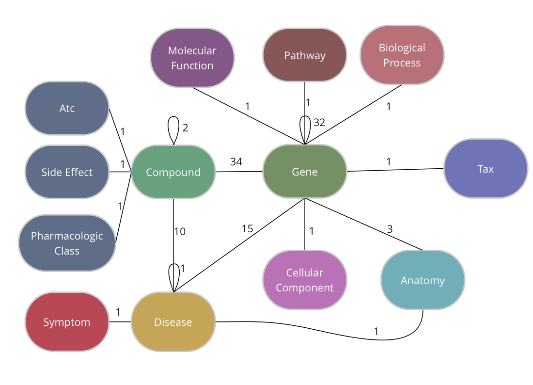
The Drug Repurposing Knowledge Graph (DRKG) is a comprehensive biological knowledge graph relating genes, compounds, diseases, biological processes, side effects and symptoms. DRKG includes information from six existing databases (DrugBank, Hetionet, GNBR, String, IntAct and DGIdb) as well as data collected from recent publications, particularly related to Covid19. It includes 97,238 entities belonging to 13 entity-types; and 5,874,261 triplets belonging to 107 edge-types. These 107 edge-types show a type of interaction between one of the 17 entity-type pairs (multiple types of interactions are possible between the same entity-pair), as depicted in the adjacent image.
The DRKG data is freely available we explain below how you can import the data into TigerGraph.

Creating the schema in TigerGraph

TigerGraph has an integrated schema designer which allows one to design a schema with ease. There is also an API to define a schema via code and since the DRKG schema has lots of edge types between some entities (Compound-Gene has 34, Gene-Gene has 32), it’s easier to do it via code. The method below, in fact, allows you to output a schema for any given dataset of triples.

The end-result inside TigerGraph can be seen in the adjacent picture and is identical to the schema above. The many reflexive edges you see are an explicit depiction of the multiple edge count above.
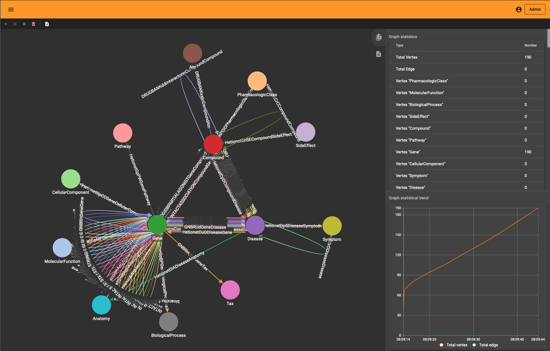
Generating the schema involves the following elements:

  1. given the triples collection, we loop over each one to harvest the endpoints (aka head and tail) and name of the relation (aka relation or predicate)
  2. the endpoints are in the form “type::id” so we split the string to extract the type and the id
  3. each node type and node id are bundled in entity collection
  4. the names of the relations are cleaned and put in a separate dictionary.

A typical relation name (e.g. “DRUGBANK::ddi-interactor-in::Compound:Compound”) contains some special characters which are not allowed in a TigerGraph schema. All of these characters are removed but this is the only difference with the initial (raw) data.

Once you have downloaded the dataset you should see a TSV file called “drkg.tsv”. This contains all the triples (head-relation-tail) and it can be loaded with a simple Pandas method:

import pandas as pd
drkg_file = './drkg.tsv'
df = pd.read_csv(drkg_file, sep="\t")
triplets = df.values.tolist()

The triplets list is a large array of 5874260 items.

Next, the recipe above output a string which one can execute inside TigerGraph; a schema creation query.

rtypes = dict() # edge types per entity-couple
entity_dic = {} # entities organized per type
for triplet in triplets:
    [h,r,t] = triplet
    h_type = h.split("::")[0].replace(" " ,"")
    h_id = str(h.split("::")[1])
    t_type = t.split("::")[0].replace(" " ,"")
    t_id = str(t.split("::")[1])

    # add the type if not present
    if not h_type in entity_dic:
        entity_dic[h_type]={}
    if not t_type in entity_dic:
        entity_dic[t_type] ={}

    # add the edge type per type couple
    type_edge = f"{h_type}::{t_type}"
    if not type_edge in rtypes:
        rtypes[type_edge]=[]
    r = r.replace(" ","").replace(":","").replace("+","").replace(">","").replace("-","")
    if not r in rtypes[type_edge]:
        rtypes[type_edge].append(r)

    # spread entities
    if not h_id in entity_dic[h_type]:
        entity_dic[h_type][h_id] = h
    if not t in entity_dic[t_type]:
        entity_dic[t_type][t_id] = t

schema = ""
for entity_type in entity_dic.keys():
    schema += f"CREATE VERTEX {entity_type} (PRIMARY_ID Id STRING) With primary_id_as_attribute=\"true\"\n"
for endpoints in rtypes:
    [source_name, target_name] = endpoints.split("::")
    for edge_name in rtypes[endpoints]:
        schema += f"CREATE DIRECTED EDGE {edge_name} (FROM {source_name}, TO {target_name})\n"
print(schema)

TigerGraph has excellent documentation and you should read through the “Defining a graph schema” topic which explains in detail the syntax used in the script above.

The output of this Python snippet (full listing here) looks like the following

CREATE VERTEX Gene (PRIMARY_ID Id STRING) With primary_id_as_attribute="true"
CREATE VERTEX Compound (PRIMARY_ID Id STRING) With primary_id_as_attribute="true"
...
CREATE DIRECTED EDGE GNBRZCompoundGene (FROM Compound, TO Gene)
CREATE DIRECTED EDGE HetionetCbGCompoundGene (FROM Compound, TO Gene)
...

You can use this directly in a GSQL interactive session or via one of the many supported languages. As described in the next section, we’ll use Python with the pyTigerGraph driver to push the schema.

Connecting and querying

Obviously, you need a TigerGraph instance somewhere and if you don’t have one around there is no easier way than via the TigerGraph Cloud.
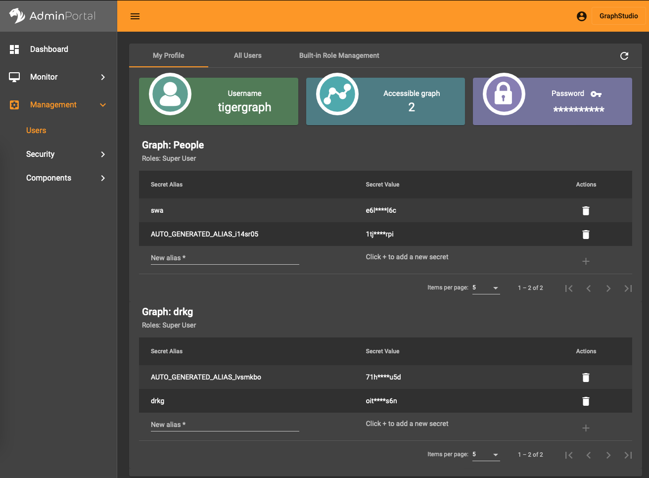
In the AdminPortal (see image) you should add a secret specific to the database. That is, you can’t use a global secret to connect, you need one per database.

Installing the pyTigerGraph drive/package is straightforward (pip install pyTigerGraph) and connecting to the database with the secret looks like the following:

import pyTigerGraph as tg
host = 'https://your-organization.i.tgcloud.io'
secret = "your-secret"
graph_name = "drkg"
user_name = "tigergraph"
password = "your-password"
token = tg.TigerGraphConnection(host=host, graphname=graph_name, username=user_name, password=password).getToken(secret, "1000000")[0]
conn = tg.TigerGraphConnection(host=host, graphname=graph_name, username=user_name, password=password, apiToken=token)

This can be condensed to just three lines but the explicit naming of the parameters is to help you get it right.

If all is well you can test the connection with

conn.echo()

which returns “Hello GSQL”. With this connection you can now use the full breadth of the GSQL query language.

In particular, we can now create the schema assembled above with this:

print(conn.gsql(
"""
    use global
    CREATE VERTEX Gene (PRIMARY_ID Id STRING) With primary_id_as_attribute="true"
    CREATE VERTEX Compound (PRIMARY_ID Id STRING) With primary_id_as_attribute="true"
    ...
    CREATE DIRECTED EDGE GNBRZCompoundGene (FROM Compound, TO Gene)
    CREATE DIRECTED EDGE HetionetCbGCompoundGene (FROM Compound, TO Gene)
...
""")

The content is a copy of the outputted string plus an extra statement use global to generate the schema in the global TigerGraph namespace. It means that the schema elements can be reused across different databases. This feature is something you will not find in any other graph database solution and has far-reaching possibilities to manage data.
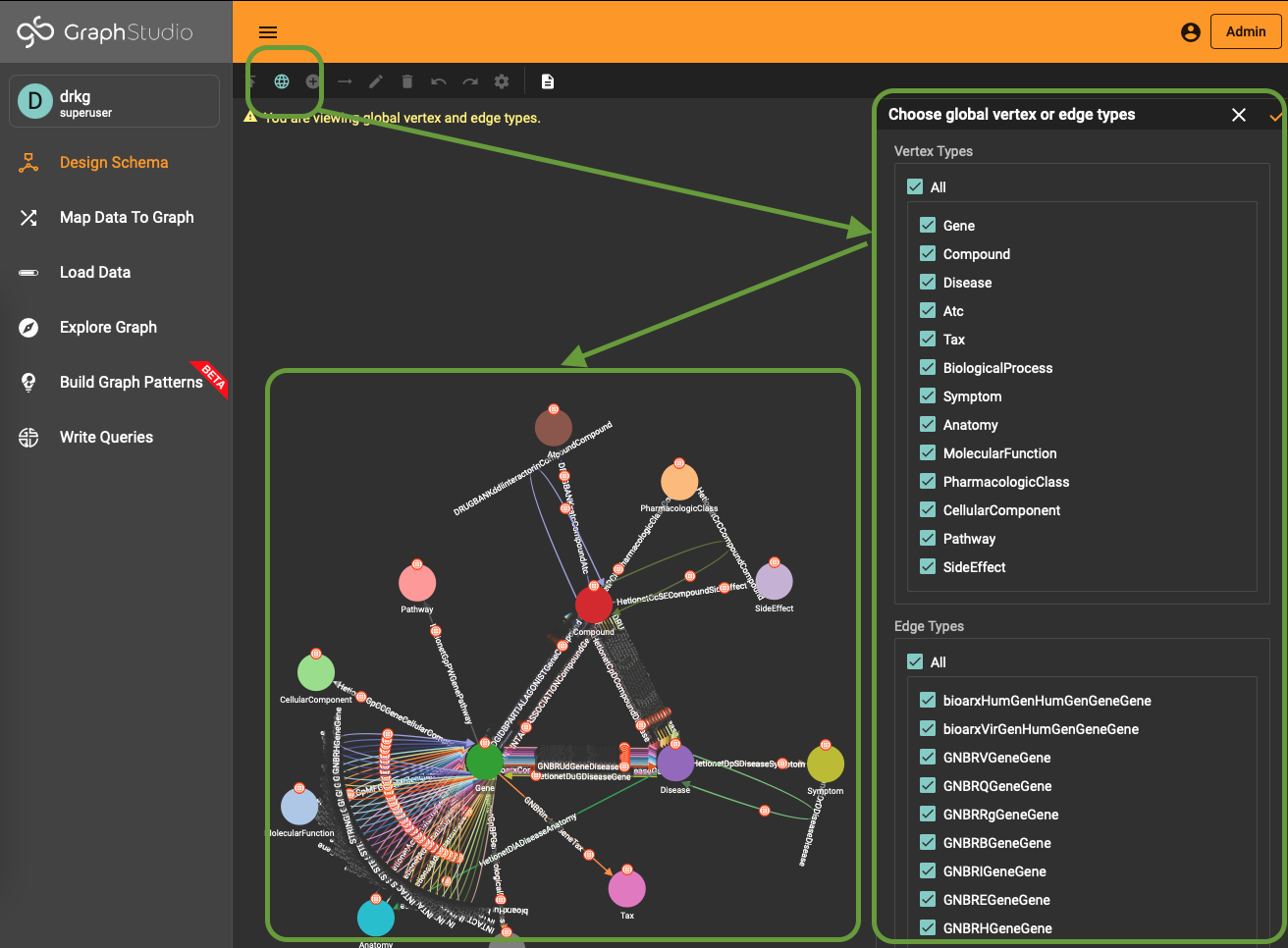
To use (part of) the global schema in a specific database you simply have to go into the database schema designer and import the elements from the global schema (see picture). Note that in the visualization you have a globe-icon to emphasize that a schema element is inherited from the global schema.

Importing the data

The Jupyter notebook to create the schema as well as to import the data can be found here.

TigerGraph has a wonderful intuitive interface to import data but the DRKG schema contains a lot of loops and the raw TSV has the node type embedded in the triple endpoints. One approach is to develop some ETL to end up with multiple files for each entity type and the relationships. The easier way is to use the REST interface to the database:

for triplet in triplets:
    [h,r,t] = triplet
    h_type = h.split("::")[0].replace(" " ,"")
    h_id = str(h.split("::")[1])
    t_type = t.split("::")[0].replace(" " ,"")
    t_id = str(t.split("::")[1])
    r = r.replace(" ","").replace(":","").replace("+","").replace(">","").replace("-","")

    conn.upsertEdge(h_type, h_id, r, t_type, t_id)

The upsertEdge method also creates the nodes if they are not present already, there is no need to upsert nodes and edges separately. This approach is much easier than the ETL one but the hidden cost is the fact that it engenders 5.8 million REST calls. In any case, creating such a large graph takes time no matter the approach.

If you are only interested in exploring things or you have limited resources, you can sample the graph and create a subgraph of DRKG fitting your needs:

amount_of_edges = 50000
triple_count = len(triplets)
sample = np.random.choice(np.arange(triple_count), amount_of_edges)
for i in sample:
    [h,r,t] = triplet
    h_type = h.split("::")[0].replace(" " ,"")
    h_id = str(h.split("::")[1])
    t_type = t.split("::")[0].replace(" " ,"")
    t_id = str(t.split("::")[1])
    r = r.replace(" ","").replace(":","").replace("+","").replace(">","").replace("-","")

    conn.upsertEdge(h_type, h_id, r, t_type, t_id)

One neat thing you’ll notice is that “Load Data” interface in TigerGraph Studio also shows the import progress if you use the REST API. You see the graph growing (to the entity and edge type level) whether you use the ETL upload or the REST import.

Exploration and Visualization

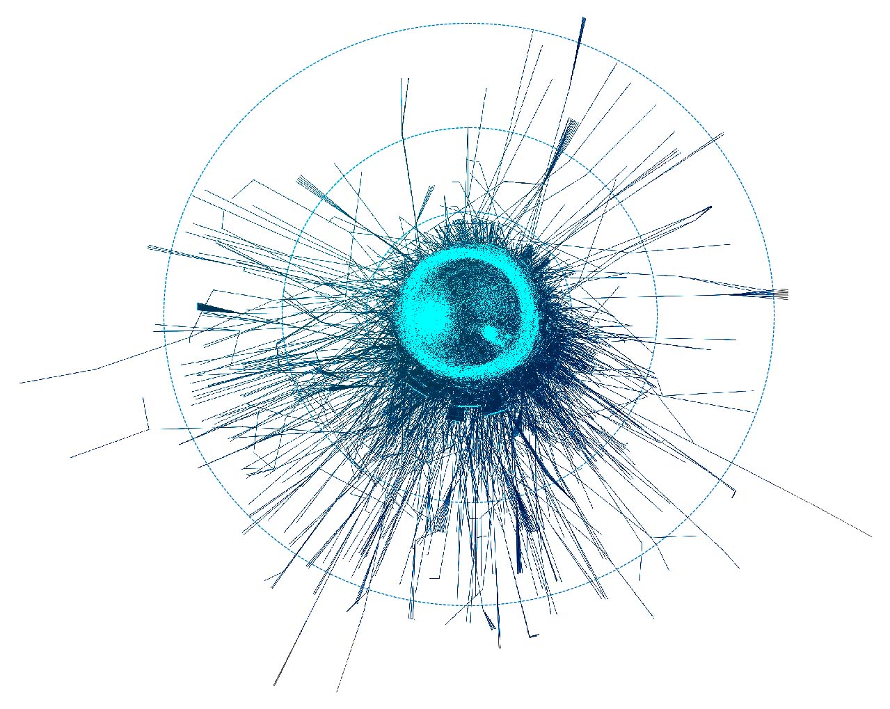
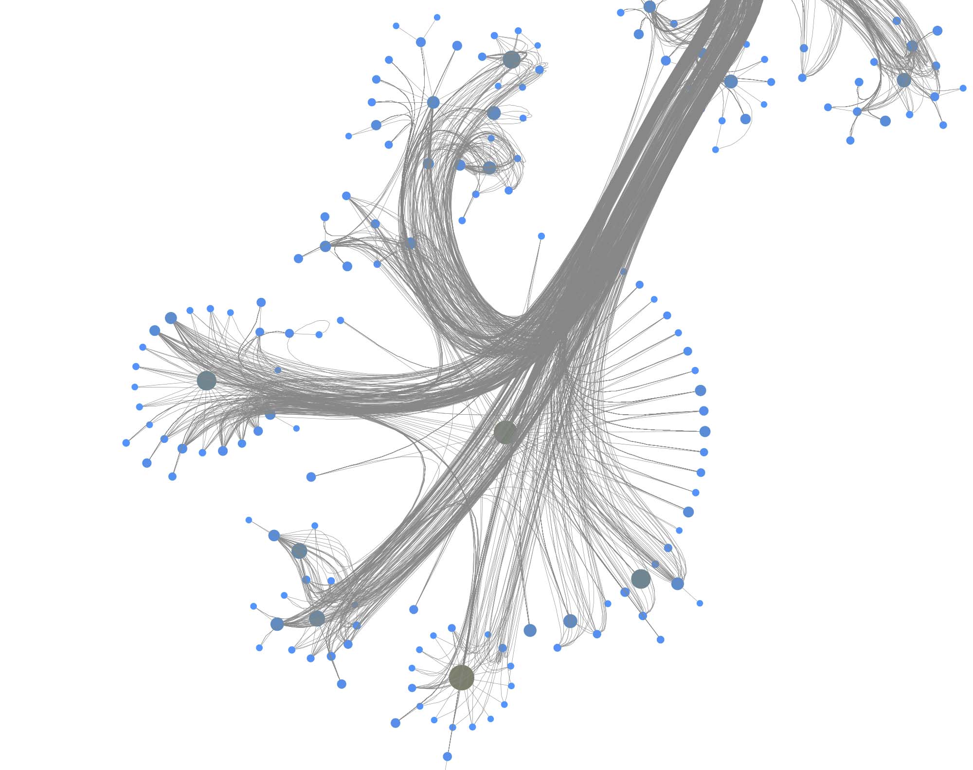
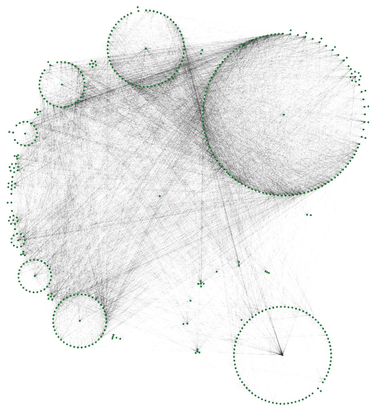
If you wonder how the DRKG graph looks like, the 0.01 ratio of node to edges automatically leads to a so-called hairball. The degree histogram confirms this and like many real-world graphs it exhibits a power-law distribution (aka scale-free network), meaning that the connectivity is mostly defined through a small set of large hubs while the mjority of the nodes has a much smaller degree.

To layout the whole graph you can use for instance the wonderful Rapids library and the force-atlas algorithm or Gephi but you will need some patience and the result will look like the image below.
Taking a subset of the whole graph reveals something more pleasing and if you hand it over to yEd Live you’ll get something like the following
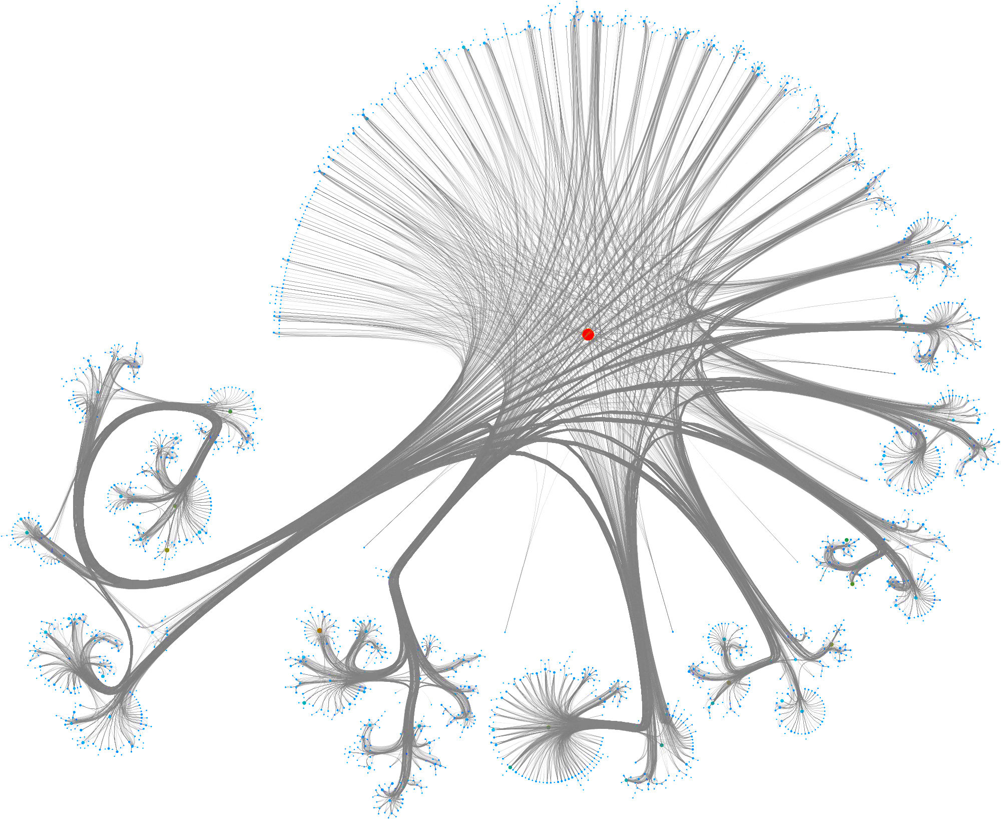
DRKG Visualization

You can furthermore use degree centrality (or any other centrality measure) to emphasize things and zooming into some of the clusters you can discover gene interactions or particular disease symptoms. Of course, all of this is just exploratory but just like any other machine learning task it’s crucial to understand a dataset and gain some intuition.
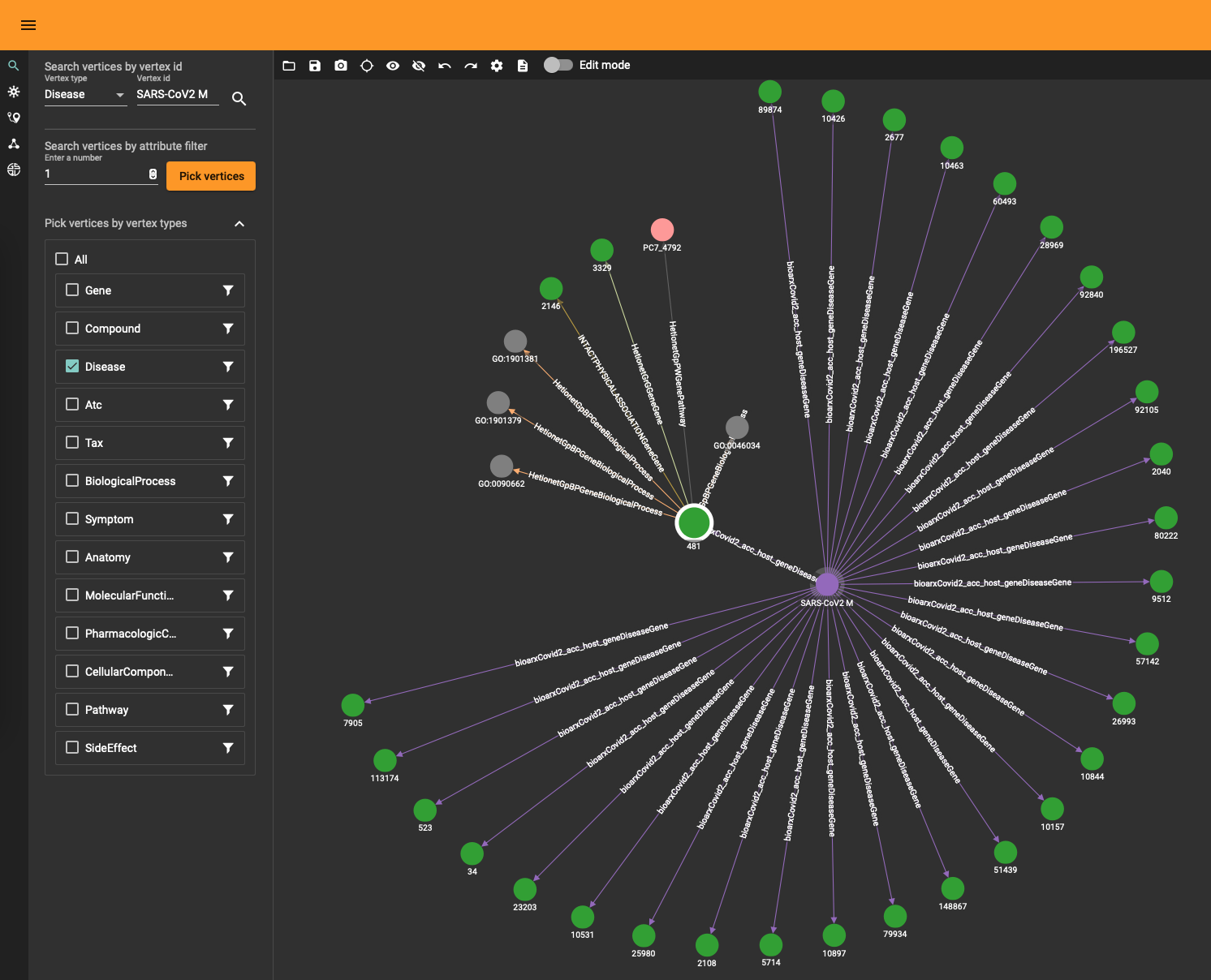
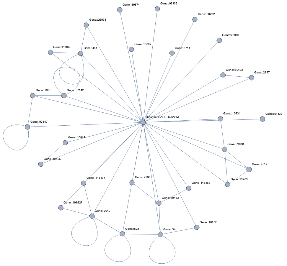
The DRKG data contains interesting information about COVID (variations). For example, the identifier “Disease::SARS-CoV2 M” refers to “severe acute respiratory syndrome coronavirus 2 membrane (M) protein” and you can use a simple GSQL query

CREATE QUERY get_covid() FOR GRAPH drkg {

    start =   {Disease.*};
    results = SELECT s FROM start:s WHERE s.id=="SARS-CoV2 M";
    PRINT results;

}

to fetch the data or use the TigerGraph data explorer. The data explorer having the advantage that you can dril down and use various layout algorithms on the fly.
Topological Link Predictions

With all the data in the graph database you can start exploring the graph. The TigerGraph GraphStudio offers various click-and-run methods to find shortest paths and other interesting insights. At the same time, the Graph Data Science Library (GDSL) has plenty of methods you can run to discover topological and other characteristics. For example, there are 303 (weakly) connected components and the largest one contains 96420 nodes while the rest are tiny islands of less than 30 nodes. This means that the gross of the data sits in the main component (consisting of 4400229 edges). You can obtain this info using GDSL using the query RUN QUERY tg_conn_comp(...) .

In the same fashion you can run GDSL methods to fetch the k-cores, the page rank and many other standard graph analytical insights. There is also a category entitled “Topological Link Prediction” and although it does what it says it’s often not sufficient to for graph completion purposes. There are various reasons for this:

  • the word “topological” refers here to the fact that the computation only takes the connectivity into account, not the potential data contained in a node or the payload on an edge. Althoug the DRKG does not have rich data inside the nodes and edges, in general one has molecular information (chemical properties), disease classes and so on. This data is in many cases at least as important as the topological one and to accurately predict new edges (or any other ML task) this data has to be included in the prediction pipeline.
  • algorithms like the Jaccard similarity only goes one level deep in searching for similarities. Of course, this has to do with algorithmic efficiency since looping over more than 5 million edges and vertex neighborhoods is demanding. In general, however, the way a node is embedded in a graph requires more than the immediate children/parents of the node.
  • topological link prediction does not infer the edge type or other data, only that an edge ‘should’ be present in a statistical sense.

At the same time one can question how meaningful it is to implement more advanced machine learning (i.e. neural networks and alike) on a database level. This remark is valid for any database, not just TigerGraph. Whether you use StarDog, SQL Server or Neo4j there some issues with embedding machine learning algorithms in a database:

  • training neural networks without the raw power of GPU processing is only possible for small datasets. Embedding graph machine learning in a database implicitly requires a way to integrate Nvidia somewhere.
  • whether you need Spark or Dask (or any other distributed processing magic) to get the job done, it leads to a whole lot of packages and requirements. Not mentioning the need to have virtual environments and all that.
  • feature engineering matters and when transforming a graph to another one (or turning it into some tabular/numpy format) you need to store things somewhere. Neo4j for example uses projections (virtual graphs) but it’s not a satisfactory solution (one cannot query projections for one).
  • there are so many ML algorithms and packages out there that it’s hardly possible to consolidate something which will answer to all business needs and graph ML tasks.

This is only to highlight that any data science library within a graph database (query language) has its limitations and that one inevitably needs to resort to a complementary solution outside the database. A typical enterprise architecture with streaming data would entail things like Apache Kafka, Amazon Kinesis, Apache Spark and all that. The general idea is as follows:

  • a representative subgraph of the graph database is extracted in function of machine learning
  • a model is trained towars the (business) goal: graph classification, link prediction, node tagging and so on
  • the model is used outside the graph database (triggered upon new graph data) and returns some new insight
  • the insight is integrated into the original graph.

In practice this involves a lot of work and some tricky questions (e.g. how to make sure updates don’t trigger the creation of existing edges) but the crux is that like so often a system should be used for what it’s made for.

With respect to drug repurposing using the DRKG graph, altough GSQL is Turing complete and hence in theory capable of running neural networks we will assemble in the next section a pipeline outside TigerGraph and feed the new insights back via a simple upsert thereafter.

Drug repurposing using Geometric Deep Learning

Graph machine learning is a set of techniques towards various graph-related tasks, to name a few:

  • graph classification: assigning a label to a while graph. For instance, determining whether a molecule (seen as a graph) is toxic or not.
  • node classification: assigning a label to a given node. For instance, inferring the gender in a social network based on given attributes.
  • link prediction (aka graph completion): predicting new edges. For instance, inferring terroristic affiliations based on social interactions and geolocation.

Drug repurposing is a special type of link prediction: it attempts to find edges between compounds and diseases which have not been considered yet. Looking at our DRKG graph it means that we are interested in edges between the Compound and Disease entity types. It doesn’t mean that other edges are of no importance. Indeed, a generic link prediction pipeline will discover patterns between arbitrary entities and one can focus equally well on new Gene-Gene interactions or symptoms indicating possible diseases.

Note that there is are many names out there to denote the same thing. Geometric (deep) learning, graph embeddings, graph neural networks, graph machine learning, non-Euclidean ML, graph signal processing… all emphasize different aspects of the same research or technology. They all have in common the use of neural networks to learn patterns in graph-like data.

On a technical level, there are heaps of frameworks and techniques with varying quality and sophistication. For drug repositioning specifically you will find the following valuable:

  • Deep Purpose A deep learning library for compound and protein modeling.
  • DRKG The data source also contain various notebooks explaining how to perform various prediction on DRKG.
  • DGL-KE Based on the DGL library, it focuses in learning large scale knowledge graphs and embeddings.
  • TorchDrug A framework designed for drug discovery.

These high-level frameworks hide a lower-level of complexity where you have more grip on assembling neural nets but it also comes with a learning curve. More specifically, PyTorch Geometric, DGL, StellarGraph and TensorFlow Geometric are the most prominent graph machine learning framework.

Crafting and training neural networks is an art and a discipline on its own. It also demands huge processing power if you have any significant dataset. In our case, the DRKG graph with its 5.8 million edges will take you days even with GPU power at your disposal. Still, if you want to train a link prediction model without lots of code, we’ll show it the next section how to proceed. Thereafter we’ll explain how you can make use of pre-trained models to bypass the demanding training phase and get straight to the drup repositioning.

How to train a link prediction model using TorchDrug

As highlighted above, you can craft your own neural net but there are nowadays plenty of high-level frameworks easing the process. TorchDrug is one such framework and it comes with lots of goodies to make one smile. As the name indicates, it’s also geared towards drug discovery, protein representation learning and biomedical graph reasoning in general.

Make sure you have PyTorch installed, as well as Pandas and Numpy. See the ‘Setup’ section below.

TorchDrug has many datasets included by default but not DRKG. It does have Hetionet, which is a subset of DRKG. Creating a dataset is, however, just a dozen lines:

import torch, os
from torch.utils import data as torch_data
from torchdrug import core, datasets, tasks, models, data, utils


class DRKG(data.KnowledgeGraphDataset):
    """
    DRKG for knowledge graph reasoning.

    Parameters:
        path (str): path to store the dataset
        verbose (int, optional): output verbose level
    """

    url = "https://dgl-data.s3-us-west-2.amazonaws.com/dataset/DRKG/drkg.tar.gz"
    md5 = "40519020c906ffa9c821fa53cd294a76"
    def __init__(self, path, verbose = 1):
        path = os.path.expanduser(path)
        if not os.path.exists(path):
            os.makedirs(path)
        self.path = path
        zip_file = utils.download(self.url, path, md5 = self.md5)
        tsv_file = utils.extract(zip_file, "drkg.tsv")
        self.load_tsv(tsv_file, verbose = verbose)

From here on you can use the whole API of TorchDrug and training a link prediction, in particular, is as simple as:

dataset = DRKG("~/data")

lengths = [int(0.8 * len(dataset)), int(0.1 * len(dataset))]
lengths += [len(dataset) - sum(lengths)]
train_set, valid_set, test_set = torch_data.random_split(dataset, lengths)

train_set, valid_set, test_set = torch_data.random_split(dataset, lengths)
print("train: ", len(train_set), "val: ", len(valid_set), "test: ", len(test_set))

model = models.RotatE(num_entity = dataset.num_entity,
                      num_relation = dataset.num_relation,
                      embedding_dim = 2048, max_score = 9)

task = tasks.KnowledgeGraphCompletion(model, num_negative = 256,
                                      adversarial_temperature = 1)

optimizer = torch.optim.Adam(task.parameters(), lr = 2e-5)
solver = core.Engine(task, train_set, valid_set, test_set, optimizer,
                      batch_size = 1024)
solver.train(num_epoch = 200)

First, a an instance of the DRKG dataset is created and it will automatically download the data to the specified directory (here, in the user’s directory ~/data) if not present already. Like any other ML task, a split of the data into training, validation and test happens next. Note that splitting a graph into separate sets is in general a non-trivial task due to edges having to be dropped in order to separate a graph. In this case, the raw data is a simple list of triples and the split is, hence, just an array split.

A semantic triple consists of a subject, a predicate and an object. This corresponds, respectively, to the three parts of an arrow: head, link and tail. In ML context you often will see (h,r,t) rather than the semantic (s,p,o) notation but the two are equivalent.

The rotatE model is an embedding of the graph using relational rotation in complex space as described here. TorchDrug has various embedding algorithms and you can read also more about this in a related article we wrote with Tomaz Bratnic. This embedding step is effectively where the neural net ‘learns’ to recognize patterns in the graph.

The link prediction task KnowledgeGraphCompletion uses the patterns recognized in the model to make predictions. This high-level method hides the tricky parts you need to master if you assemble a net manually.

Finally, the net is trained and this does not differ much from any Torch learning loop (or any other deep learning process for that matter). The number of epochs refers to how many times the data is ‘seen’ by the net and a single epoch can take up to an hour with a K80 Nvidia GPU. The large number of edges is of course the culprit here. If you want to fully train the net with an acceptable accuracy (technically, a cross-entropy below 0.2) you will need patience or a special budget. This is the reason that pretrained models are a great shortcut and the situation is similar, for example, with NLP transformers like GPT3 where it often doesn’t make sense to train a model from scratch but rather make stylistic variations of an existing one.

Drug repositioning the easy way

Just like there are various pre-trained models for NLP tasks, you can find embeddings for public datasets like DRKG. A pre-trained model for DRKG consists of vectors for each node and each edge, representing the graph elements in a (high-dimensional) vector space (also know as latent space). These embeddings can exist on their own without the need to deserialize the data back into a model, like the rotatE model above. The (node or edge) vectors effectively capture all there is to know about both the way they sit in the graph (i.e. purely topological information) and their payload (attributes or properties). Typcally, the more two vectors are similar, the more the nodes are similar in a conceptual sense. There are many ways to define ‘similar’ just like there are many ways to define distance in a topological vector space but this is beyond the scope of this article.

To be concrete, we’ll focus on finding new compounds to treat hypertension. In the DRKG graph this corresponds to node with identifier “Disease::DOID:10763”.

The possible edges can have one of the following two labels:

allowed_labels = ['GNBR::T::Compound:Disease','Hetionet::CtD::Compound:Disease']

Furthermore, we will only accept FDA approved compounds to narrow down the options:

allowed_drug = []
with open("./FDAApproved.tsv", newline='', encoding='utf-8') as csvfile:
    reader = csv.DictReader(csvfile, delimiter='\t', fieldnames=['drug','ids'])
    for row_val in reader:
        allowed_drug.append(row_val['drug'])

giving around 2100 possible compounds.

Pretrained models (well, models and graphs in general) don’t work well with concrete names but have numerical identifiers, so one needs a mapping between an actual entity name and a numerical identifier. So, you’ll often find a pretrained model file sitting next to a coupld of dictionaries:

# path to the dictionaries
entity_to_id = './entityToId.tsv'
relation_to_id = './relationToId.tsv'

entity_name_to_id = {}
entity_id_to_name = {}
relation_name_to_id = {}

with open(entity_to_id, newline='', encoding='utf-8') as csvfile:
    reader = csv.DictReader(csvfile, delimiter='\t', fieldnames=['name','id'])
    for row_val in reader:
        entity_name_to_id[row_val['name']] = int(row_val['id'])
        entity_id_to_name[int(row_val['id'])] = row_val['name']

with open(relation_to_id, newline='', encoding='utf-8') as csvfile:
    reader = csv.DictReader(csvfile, delimiter='\t', fieldnames=['name','id'])
    for row_val in reader:
        relation_name_to_id[row_val['name']] = int(row_val['id'])


allowed_drug_ids = []
disease_ids = []
for drug in allowed_drug:
    allowed_drug_ids.append(entity_name_to_id[drug])

for disease in what_diseases:
    disease_ids.append(entity_name_to_id[disease])

allowed_relation_ids = [relation_name_to_id[treat]  for treat in allowed_labels]

Now we are good to load the pretrained vectors:

entity_emb = np.load('./entity_vectors.npy')
rel_emb = np.load('./relation_vectors.npy')

allowed_drug_ids = torch.tensor(allowed_drug_ids).long()
disease_ids = torch.tensor(disease_ids).long()
allowed_relation_ids = torch.tensor(allowed_relation_ids)

allowed_drug_tensors = torch.tensor(entity_emb[allowed_drug_ids])
allowed_relation_tensors = [torch.tensor(rel_emb[rid]) for rid in allowed_relation_ids]

The entity embedding consists of 97238 vectors, matching the amount of nodes in DRKG. Complementary to this, the relation embedding consists of 107 for the 107 types of edges in DRKG. The hypertension node identifer is 83430 corresponding to “Disease::DOID:10763” label.

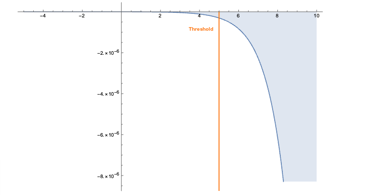
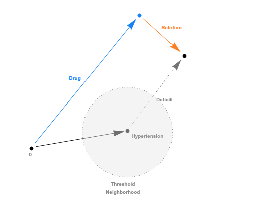
The embeddings can now be used with a standard (Euclidean) metric but to differentiate fitness it’s often more convenient to use a measure which penalizes long distances. It’s a bit like molcular interaction forces (the so-called Lennard-Jones potential)where only the short range matters. This scoring measure (shown In the plot below) quickly diverges beyond a threshold which can be set to accept more or fewer drugs. In the context of differential geometry one would speak of curvature as a measure of deficit between two parallel transports. If the deficit vector is within the threshold neighborhood it’s accepted as a treatment, otherwise the score quickly fades to large values. The fact that the score is negative is simply an easy way to sort the results. The closer the score it to zero the more it’s a perfect fit to treat hypertension.
In code this idea is simply this:

threshold= 20
def score(h, r, t):
    return fn.logsigmoid(threshold - torch.norm(h + r - t, p=2, dim=-1))

allowed_drug_scores = []
drug_ids = []
for relation_tensor in range(len(allowed_relation_tensors)):
    rel_vector = allowed_relation_tensors[relation_tensor]
    for disease_id in disease_ids:
        disease_vector = entity_emb[disease_id]
        drug_score = score(allowed_drug_tensors, rel_vector, disease_vector)
        allowed_drug_scores.append(drug_score)
        drug_ids.append(allowed_drug_ids)
scores = torch.cat(allowed_drug_scores)
drug_ids = torch.cat(drug_ids)

Finally, the compound/drugs found are collected and the identifier converted back to actual labels. The result is

Compound::DB00584	-1.883488948806189e-05
Compound::DB00521	-2.2053474822314456e-05
Compound::DB00492	-2.586808113846928e-05
...

and the most likely candidate is Enalapril (DB00584 is the DrugBank Accession Number) which can be checked as a actual drug to treat hypertension.

You should note that with the code above you only have to alter the disease identifier to extract a prediction for that particular disease. Using the Drug Bank you can look up the Accession Number, if necessary.

Another important things to emphasize is the sheer speed with which predictions are made thanks to the pretrained vectors. In effect, you can hook this up via triggers to automatically make prediction when the knowledge graph is changed. Such a setup would be similar to what one designs for fraud detection and, in general, realtime anomaly detection of transactions. Feeding back the link predictions to TigerGraph is really just a REST call away.

Challenges

The small amount of code necessary to achieve all this hides a lot of sophisticated machine learning under the hood. To correctly design and train a graph machine learning pipeline on top of DRKG requires, as mentioned earlier, a lot of time and GPU power. Although the knowledge graph contains plenty of valuable information, it’s all topological. That is, the nodes and edges don’t contain any data and a much more refined drug repurposing model would be possible if e.g. molecular properties, symptom details and other data would be included. This would, however, engender the creation of more complext neural net and more data would mean longer training times (more epochs).

There are also a number of non-technical downsides to drug repositioning:

  • the dosage required for the treatment of a disease usually differs from that of its original target disease, and if this happens, the discovery team will have to begin from Phase I clinical trials. This effectively strips drug repurposing of its advantages over classic drug discovery.
  • no matter how big the knowledge graph is, nothing replaces the expertise and scientific know-how of professionals. Obviously, one shouldn’t narrow down the discovery of treatments and compounds to an algorithm. Graph machine learning is an incentive, not a magic wand.
  • patent right issues can be very complicated for drug repurposing due to the lack of experts in the legal area of drug repositioning, the disclosure of repositioning online or via publications, and the extent of the novelty of the new drug purpose. See the article “Overcoming the legal and regulatory barriers to drug repurposing” for a good overview.

References

Books:

Articles:

TigerGraph:

Data:

  • DRKG The 5.8 million triples a click away.
  • Drug Bank Drug database and more.
  • Clinical Trials ClinicalTrials.gov is a database of privately and publicly funded clinical studies conducted around the world.

Frameworks:

  • Deep Purpose A Deep Learning Library for Compound and Protein Modeling DTI, Drug Property, PPI, DDI, Protein Function Prediction.
  • DGL Easy deep learning on graphs.
  • TorchDrug Easy drug discovery (and much more).
  • StellarGraph Wonderful generic graph machine learning package.
  • PyTorch Geometric Pretty much the de facto deep learning framework.
  • TensorFlow Geometric Similar to PyTorch, but a bit late to the party (ie. more recent and less mature).

Setup

All the files you need are in the Github repo except for the two files containing the pretrained vectors (you can find them here).

Make sure you have Python installed (at least 3.8 and at least 3.9 if you have Apple Silicon) as well as TorchDrug, Numpy and Pandas. Of course, you better have all this in a separate environment.

conda create --name repurpose python=3.9
conda activate repurpose
conda install numpy pandas pyTigerGraph
conda install pytorch -c pytorch
pip install torchdrug
conda install jupyter

Create a free TigerGraph database and for this database create a secret as described above. Check that you can connect to your database with something like this

import pyTigerGraph as tg
host = 'https://your-organization.i.tgcloud.io'
secret = "your-secret"
graph_name = "drkg"
user_name = "tigergraph"
password = "your-password"
token = tg.TigerGraphConnection(host=host, graphname=graph_name, username=user_name, password=password).getToken(secret, "1000000")[0]
conn = tg.TigerGraphConnection(host=host, graphname=graph_name, username=user_name, password=password, apiToken=token)
conn.echo()

You don’t have to download the DRKG data if you use the torchDrugModel.py file since it will download it for you. If you want to download the data to upload to TigerGraph, use this file.

The CreateSchema.ipynb notebook will help you upload the TigerGraph schema and the hypertensionRepositioning.ipnb notebook contains the code described in this article.
A graph database is one that stores data in terms of entities and the relationships between entities. A variant on this theme are RDF (resource description framework) databases which store data in the format subject-predicate-object, which is known as a triple.

There are three types of graph database: true graph databases, triple stores and conventional databases that provide some graphical capabilities. Triple stores are often referred to as RDF or semantic databases. The difference between a true graph product and a triple store is that the former supports index free adjacency (which means you can traverse a graph without needing an index) and the latter doesn’t. The former are designed to support property graphs (graphs where properties may be assigned to either entities or their relationships, or both) but recently some triple stores have added this capability.

Both graph and RDF databases may be native products or they may be built on top of other database types. Most commonly, other database types are forms of NoSQL database though there are some relational implementations.

RDF databases target semantic processing, often with the ability to combine information across structured and unstructured data. Both graph and RDF databases may be ACID compliant and both are frequently targeted at transactional environments. All graph products target analytics but different products are targeted at operational analytics (those suitable for transactional environments) as opposed to data warehousing analytics. In this last category there is also a distinction between vendors targeting known-known problems as opposed to those that also cover known-unknowns and those tackling unknown-unknowns: the most intractable of all.

Given that both graph and RDF databases target both transactional environments and have query processing capabilities, these are an obvious candidate for supporting so-called HTAP processing whereby the database is used for both transactional/operational processing and real-time analytics. Compared to some other approaches to HTAP this has the major advantage that the data only needs to be stored once. Both concurrent analytics (where the analytics is separate from operational processes, for example in supporting real-time dashboards) and in-process analytics (where the analytics are embedded in real-time operational processing) may be supported. In the latter case, there are a variety of graph 

algorithms supported by vendors that may be implemented for machine learning purposes.

Graph databases handle a class of issues that are too structured for NoSQL and too diverse for relational technologies. In the latter case, relational databases are inherently limited to one-to-one, many-to-one and one-to-many relationships. They do not cater well for problems (such as bill of materials – a classic case) that are many-to-many. For these types of requirements graph databases not only perform way better better than relational databases but they allow some types of query that are simply not possible otherwise. Semantic query support tends to be particularly strong in triple stores.

Another major point is that research suggests that graph visualisations are very easy and intuitive for users. It is also worth noting that many (not all) graph products are schema-free. This means that if you want to change the structure of the environment you simply add a new entity or relationship as required and do not have to explicitly implement a schema change. This is a major advantage over relational databases.

This market is emerging and there are many open source projects and vendors, many of which will not ultimately survive. Nevertheless there are still new products coming on to the marketplace. Conversely, there are companies that have been in this space for more than a decade, so the technology is not entirely new. One noticeable trend is for triple store vendors to add support for property graphs.

Another trend is towards multi-model implementations. This is where the database supports graph technology as just one of possibly several views into the data. A major consideration with such offerings is the extent to which these different representations can work together. Some vendors require, for example, require a different API to be used for each model type supported, whereas others have integrated their environment so that the different models are effectively transparent to one another.

One major issue that has yet to be finalised is with respect to language support. SPARQL (SPARQL protocol and RDF query language) is a W3C standard and is a declarative language but by no means all vendors support it. In general, RDF vendors support SPARQL, but property graph vendors do not, though there are exceptions to this. In the property graph space the 

Gremlin graph traversal language is part of the Apache Tinkerpop project and is supported by some vendors, while other suppliers have adopted their own “SQL-like” languages. Also with significant traction is OpenCypher, which is a declarative language (Gremlin is only partially so). ANSI has a working party to define SQL extensions to support graph processing while there is also an initiative to create a standardised GQL (graph query language). It is also worth noting that GraphQL, which is an open source project, is gaining traction as a graph API to replace REST.

Finally, while it is too early to call this trend one vendor has introduced a graph capability based on adjacency matrices rather than adjacency lists. If this proves successful, and early results suggest that that will be the case, then we are like to see this being more widely adopted as it promises much better performance.

There have been a lot of new entrants to the market and changes amongst those within the market. As far as new products are concerned these include RedisGraph, TigerGraph, MemGraph, Trovares, and Microsoft Cosmos DB. Cambridge Semantics has unbundled AnzoGraph from its Anzo Data Lake offering and both Amazon and SAP have also entered the market. In the case of Amazon Neptune, it is an open secret that this is based on BlazeGraph while SAP has acquired OrientDB. Or, rather, it acquired the company that had acquired OrientDB, though we think that OrientDB was probably incidental as far as this acquisition was concerned. Nevertheless, SAP appears to be moving ahead with the product though there is the perennial danger that it may increasingly be targeted at the SAP user base rather than the wider community.

The one company that has withdrawn from the graph space is IBM. However, the company continues to work on the development of JanusGraph (effectively a replacement to Titan).

Despite all of the above, the market leaders in this space continue to be Neo4J and OntoText (GraphDB), which are graph and RDF database providers respectively. These are the longest established vendors in this space (both founded in 2000) so they have a longevity and experience that other suppliers cannot yet match. How long this will remain the case remains to be seen.

If you want to play with SPARQL and triples you will find that you end up with a few options: Apache Jena (Fuseki), Stardog and BrightstarDB. It seems that BrighstarDB is not active anymore and the free version of Stardog is limited to millions of triples. In one of our projects we used Fuseki for a POC and found it to be OK until we hit various incomprehensible problems and loss of data. To be clear: do not use Apache Jena beyond a POC and simple setups. The problem is that you will not find any other SPARQL open source alternative and, hence, forced to buy expensive licenses.

Considering that Jena is relatively old and widely known one would think that it’s battle resistant and though it does not boast enterprise features (e.g. clustering) it should be good to go. Not. For instance:

  • we found that concurrent reading and writing of triples would bring the service to a halt with as little as three users
  • reading after writing sometimes requires one to insert a delay in order to let Jena digest the changes
  • deleted databases persist on disk while not visible in Jena
  • data sometimes disappears for no reason

and one cannot but systematically distrust the service. Some of the issues likely have their origin in Fuseki (the REST service on top of Jena) but others definitely are deep inside Jena. This situation adds to the problematic acceptance of semantic thinking in the industry. Ontologies and related tools (like Stanford’s Protégé) still very much feel like academic inventions and although there is a growing interest it’s still far away from the relational standard. A bit like the R language for statistical analysis; massive value but quirky at its core.

So, using open source triple stores for real-world applications? Not yet. If your triple count is in the trillions you will have to go for MarkLogic and alike. Which is really a shame since there are so many great open source or free solutions in the relational world.

A very promising product in a crowded market with unique features. Not enterprise ready yet but could be in a year and provided it grows in the right way (or with the right guidance) a company well worth keeping an eye on.

On knowledge representation through ontology logs and how it’s related to category theory.

A multi-part series on knowledge graph modeling aka semantics and related technologies.

A multi-part series on knowledge graph modeling aka semantics and related technologies.