Embedding of nodes happens via word2vec by means of a smart trick: using randomg walks over the graph to generate ‘word’ sequences.
Stellargraph has its own direct method to perform the embedding but the intermediate methods highlights better the process. So, below we generate the node2vec embedding via an explicit walk and show how it generates a really good community detection separation.

    import networkx as nx
    import numpy as np
    import matplotlib.pyplot as plt
    from sklearn.manifold import TSNE
    %matplotlib inline

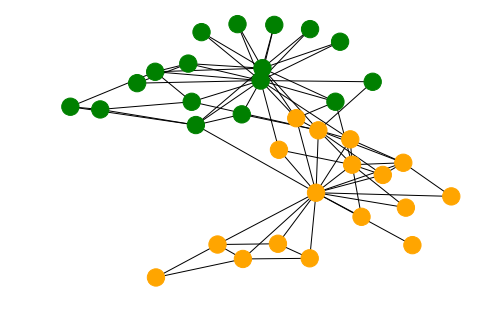
We’ll use the karater club to demonstrate the process. The graph consists of two sets of nodes which are a well-separated according to the ‘club’ property.

    g_nx = nx.karate_club_graph()
    cols = ["green" if g_nx.nodes[n]["club"]=='Officer' else "orange" for n in g_nx.nodes()]
    nx.draw(g_nx, node_color=cols)

From this graph we create a Stellargraph and perform a biased random walk on it. This generates word sequences, in this case the string value of the node index.

    from stellargraph.data import BiasedRandomWalk
    from stellargraph import StellarGraph
    from gensim.models import Word2Vec
    rw = BiasedRandomWalk(StellarGraph(g_nx))
    walks = rw.run(
          nodes=list(g_nx.nodes()), # root nodes
          length=100,  # maximum length of a random walk
          n=10,        # number of random walks per root node
          p=0.5,       # Defines (unormalised) probability, 1/p, of returning to source node
          q=2.0        # Defines (unormalised) probability, 1/q, for moving away from source node
    )
    walks = [list(map(str, walk)) for walk in walks]
    model = Word2Vec(walks, size=128, window=5, min_count=0, sg=1, workers=2, iter=1)

The value of an embedding is for instance

    model.wv['29']
array([ 0.0283457 ,  0.06906749, -0.09740856,  0.08761664,  0.0240158 ,
       -0.04252268,  0.05366189,  0.12255755, -0.14192946, -0.12441556,
        0.14022443,  0.16821992,  0.01899681,  0.02525605, -0.129657  ,
       -0.00075872, -0.10963597, -0.24603637,  0.14481993,  0.04069758,
       ...
       -0.03686432,  0.28888953,  0.06754036], dtype=float32)

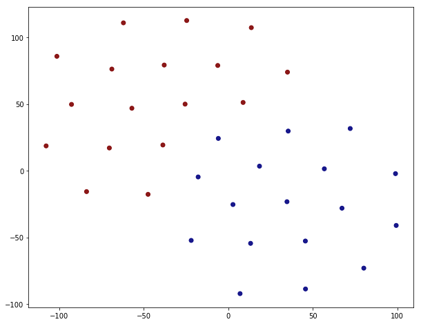
In order to visualize the embedding one has to somehow reduce the dimension. This is most easily done via t-SNE.

    # Retrieve node embeddings and corresponding subjects
    node_ids = model.wv.index2word  # list of node IDs
    node_embeddings = model.wv.vectors  # numpy.ndarray of size number of nodes times embeddings dimensionality
    node_targets = [ g_nx.node[int(node_id)]['club'] for node_id in node_ids]
    # Apply t-SNE transformation on node embeddings
    tsne = TSNE(n_components=2)
    node_embeddings_2d = tsne.fit_transform(node_embeddings)
    alpha=0.9
    label_map = { l: i for i, l in enumerate(np.unique(node_targets))}
    node_colours = [ label_map[target] for target in node_targets]
    plt.figure(figsize=(10,8))
    plt.scatter(node_embeddings_2d[:,0],
                node_embeddings_2d[:,1],
                c=node_colours, cmap="jet", alpha=alpha)
<matplotlib.collections.PathCollection at 0x1463cfc50>

This looks like a clean separation indeed. The splitting is not 100% correct though, just by looking at the corresponding value of the ‘club’ property.

    [g_nx.nodes[i] for i,v in enumerate(node_colours) if v==1]
[{'club': 'Mr. Hi'},
 {'club': 'Mr. Hi'},
 {'club': 'Mr. Hi'},
 {'club': 'Officer'},
 {'club': 'Mr. Hi'},
 {'club': 'Officer'},
 {'club': 'Officer'},
 {'club': 'Officer'},
 {'club': 'Mr. Hi'},
 {'club': 'Officer'},
 {'club': 'Officer'},
 {'club': 'Officer'},
 {'club': 'Officer'},
 {'club': 'Officer'},
 {'club': 'Officer'},
 {'club': 'Officer'},
 {'club': 'Officer'}]

Five out of senteen are incorrect. This is still remarkable considering the fact that node2vec process did not know anything at about the ‘club’ property but that it’s an emergent feature of the embedding.