
Updated November 2022
The code in this article can be found in this Colab notebook .
NetworkX is a graph analysis library for Python. It has become the standard library for anything graphs in Python. In addition, it’s the basis for most libraries dealing with graph machine learning. Stellargraph, in particular, requires an understanding of NetworkX to construct graphs.
Below is an overview of the most important API methods. The official documentation is extensive but it remains often confusing to make things happen. Some simple questions (adding arrows, attaching data…) are usually answered in StackOverflow, so the guide below collects these simple but important questions.
General remarks
The library is flexible but these are my golden rules:
- do not use objects to define nodes, rather use integers and set data on the node. The layout has issues with objects.
- the API changed a lot over the versions, make sure when you find an answer somewhere that it matches your version. Often methods and answers do not apply because they relate to an older version.
- if you wish to experiment with NetworkX in Jupyter, go for Colab and use this stepping stone:
!pip install faker
import networkx as nx
import matplotlib.pyplot as plt
from faker import Faker
faker = Faker()
%matplotlib inline
Creating graphs
There are various constructors to create graphs, among others:
# default
G = nx.Graph()
# an empty graph
EG = nx.empty_graph(100)
# a directed graph
DG = nx.DiGraph()
# a multi-directed graph
MDG = nx.MultiDiGraph()
# a complete graph
CG = nx.complete_graph(10)
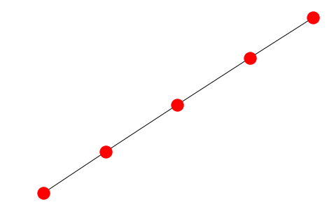
# a path graph
PG = nx.path_graph(5)
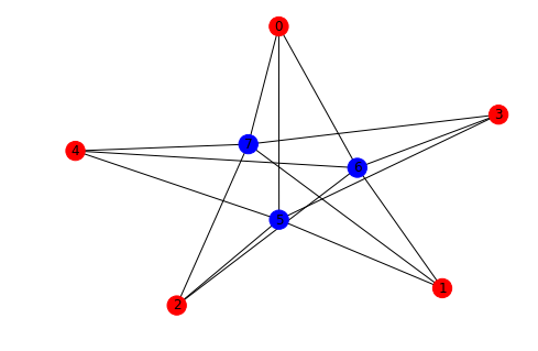
# a complete bipartite graph
CBG = nx.complete_bipartite_graph(5,3)
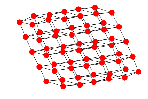
# a grid graph
GG = nx.grid_graph([2, 3, 5, 2])
Make sure you understand each class and the scope of each. Certain algorithms, for instance, work only with undirected graphs.
Graph generators
Graph generators produce random graphs with particular properties which are of interest in the context of statistics of graphs. The best-known phenomenon is six degrees of separation which you can find on the internet, our brains, our social network and whatnot.
Erdos-Renyi
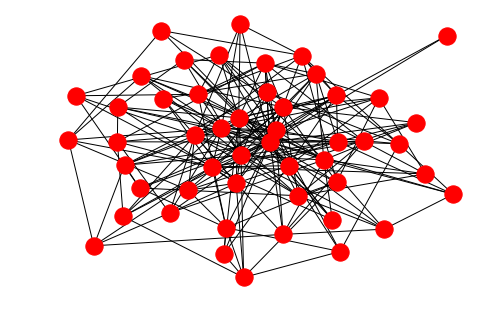
The Erdos-Renyi model is related to percolations and phase transitions but is in general the most generic random graph model.
The first parameter is the amount of nodes and the second a probability of being connected to another one.
er = nx.erdos_renyi_graph(50, 0.15)
nx.draw(er, edge_color='silver')
Watts-Strogratz
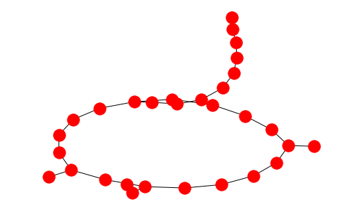
The Watts-Strogratz model produces small-world properties. The first parameter is the amount of node then follows the default degree and thereafter the probability of rewiring and edge. So, the rewiring probability is like the mutation of an otherwise fixed-degree graph.
ws = nx.watts_strogatz_graph(30, 2, 0.32)
nx.draw(ws)
Barabasi-Albert
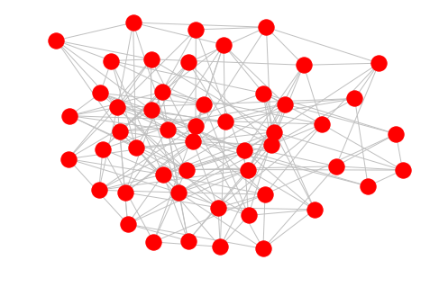
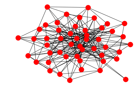
The Barabasi-Albert model reproduces random scale-free graphs which are akin to citation networks, the internet and pretty much everywhere in nature.
ba = nx.barabasi_albert_graph(50, 5)
nx.draw(ba)
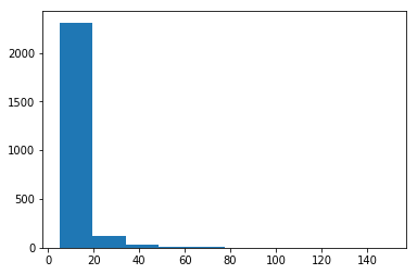
You can easily extract the exponential distribution of degrees:
g = nx.barabasi_albert_graph(2500, 5)
degrees = list(nx.degree(g))
l = [d[1] for d in degrees]
plt.hist(l)
plt.show()
Drawing graphs
The draw method without additional will present the graph with spring-layout algorithm:
nx.draw(PG)
There are of course tons of settings and features and a good result is really dependent on your graph and what you’re looking for. If we take the bipartite graph for example it would be nice to see the two sets of nodes in different colors:
from networkx.algorithms import bipartite
X, Y = bipartite.sets(CBG)
cols = ["red" if i in X else "blue" for i in CBG.nodes() ]
nx.draw(CBG, with_labels=True, node_color= cols)
The grid graph on the other hand is better drawn with the Kamada-Kawai layout in order to see the grid structure:
nx.draw_kamada_kawai(GG)
Nodes
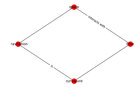
If you start from scratch the easiest way to define a graph is via the add_edges_from method as shown here:
G = nx.Graph()
G.add_node("time")
G.add_edges_from([
    ("time","space"),
    ("gravitation","curvature"),
    ("gravitation","space"),
    ("time","curvature"),
    ])
labels = {}
pos = nx.layout.kamada_kawai_layout(G)
nx.draw(G, pos=pos, with_labels= True)
nx.draw_networkx_edge_labels(G,pos,
    {
        ("time","space"): "interacts with",
        ("gravitation","curvature"): "is"
    },
    label_pos=0.4
)
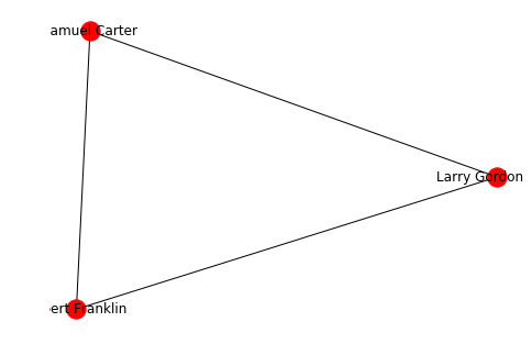
The nodes can however be arbitrary objects:
from faker import Faker
faker = Faker()
class Person:
    def __init__(self, name):
        self.name = name
    @staticmethod
    def random():
        return Person(faker.name())

g = nx.Graph()
a = Person.random()
b = Person.random()
c = Person.random()
g.add_edges_from([(a,b), (b,c), (c,a)])
# to show the names you need to pass the labels
nx.draw(g, labels = {n:n.name for n in g.nodes()}, with_labels=True)
As mentioned earlier, it’s better to use numbers for the nodes and set the data via the set_node_attributes methods as shown below.
Edges
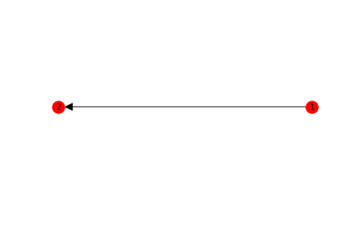
Arrows can only be shown if the graph is directed. NetworkX is essentially a graph analysis library and much less a graph visualization toolbox.
G=nx.DiGraph()
G.add_edge(1,2)
pos = nx.circular_layout(G)
nx.draw(G, pos, with_labels = True , arrowsize=25)
plt.show()
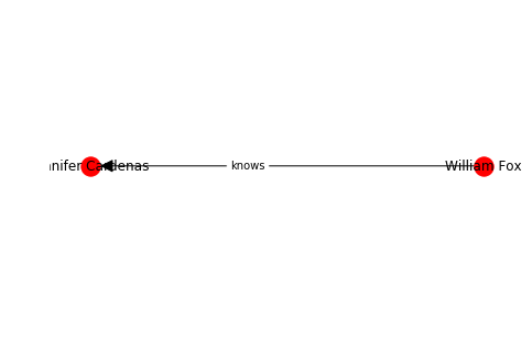
Data can be assigned to an edge on creation
G = nx.DiGraph()
a = Person.random()
b = Person.random()
G.add_node(0, data=a)
G.add_node(1, data=b)
G.add_edge(0, 1, label="knows")
labelDic = {n: G.nodes[n]["data"].name for n in G.nodes()}
edgeDic = {e: G.get_edge_data(*e)["label"] for e in G.edges}
kpos = nx.layout.kamada_kawai_layout(G)
nx.draw(G, kpos,  labels=labelDic, with_labels=True, arrowsize=25)
nx.draw_networkx_edge_labels(G, kpos, edge_labels=edgeDic, label_pos=0.4)
Analysis
There many analysis oriented methods in NetworkX, below are just a few hints to get you started.
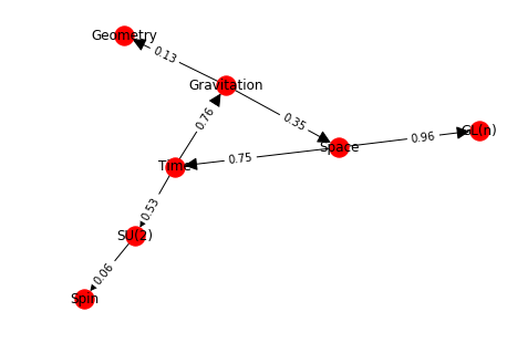
Let’s assemble a little network to demonstrate the methods:
import random

gr = nx.DiGraph()
gr.add_node(1, data={'label': 'Space'})
gr.add_node(2, data={'label': 'Time'})
gr.add_node(3, data={'label': 'Gravitation'})
gr.add_node(4, data={'label': 'Geometry'})
gr.add_node(5, data={'label': 'SU(2)'})
gr.add_node(6, data={'label': 'Spin'})
gr.add_node(7, data={'label': 'GL(n)'})
edge_array = [(1, 2), (2, 3), (3, 1), (3, 4), (2, 5), (5, 6), (1, 7)]
gr.add_edges_from(edge_array)
for e in edge_array:
    nx.set_edge_attributes(gr, {e: {'data':{'weight': round(random.random(),2)}}})
    gr.add_edge(*e, weight=round(random.random(),2))
    labelDic = {n:gr.nodes[n]["data"]["label"] for n in gr.nodes()}
    edgeDic = {e:gr.edges[e]["weight"] for e in G.edges}
kpos = nx.layout.kamada_kawai_layout(gr)
nx.draw(gr,kpos,  labels = labelDic, with_labels=True, arrowsize=25)
o=nx.draw_networkx_edge_labels(gr, kpos, edge_labels= edgeDic, label_pos=0.4)
Getting the adjacency matrix gives a sparse matrix. You need to use the todense method to see the dense matrix. There is also a to_numpy_matrix method which makes it easy to integrate with numpy mechanics:
nx.adjacency_matrix(gr).todense()
giving:
matrix([[0.  , 0.41, 0.  , 0.  , 0.  , 0.  , 0.64],
        [0.  , 0.  , 0.28, 0.  , 0.53, 0.  , 0.  ],
        [0.47, 0.  , 0.  , 0.65, 0.  , 0.  , 0.  ],
        [0.  , 0.  , 0.  , 0.  , 0.  , 0.  , 0.  ],
        [0.  , 0.  , 0.  , 0.  , 0.  , 0.27, 0.  ],
        [0.  , 0.  , 0.  , 0.  , 0.  , 0.  , 0.  ],
        [0.  , 0.  , 0.  , 0.  , 0.  , 0.  , 0.  ]])
The spectrum of this adjacency matrix can be directly obtained via the adjacency_spectrum method:
nx.adjacency_spectrum(gr)
array([-0.18893681+0.32724816j, -0.18893681-0.32724816j,
        0.37787363+0.j        ,  0.        +0.j        ,
        0.        +0.j        ,  0.        +0.j        ,
        0.        +0.j        ])
The Laplacian matrix (see definition here) is only defined for undirected graphs but is just a method away:
nx.laplacian_matrix(gr.to_undirected()).todense()
matrix([[ 1.52, -0.41, -0.47,  0.  ,  0.  ,  0.  , -0.64],
        [-0.41,  1.22, -0.28,  0.  , -0.53,  0.  ,  0.  ],
        [-0.47, -0.28,  1.4 , -0.65,  0.  ,  0.  ,  0.  ],
        [ 0.  ,  0.  , -0.65,  0.65,  0.  ,  0.  ,  0.  ],
        [ 0.  , -0.53,  0.  ,  0.  ,  0.8 , -0.27,  0.  ],
        [ 0.  ,  0.  ,  0.  ,  0.  , -0.27,  0.27,  0.  ],
        [-0.64,  0.  ,  0.  ,  0.  ,  0.  ,  0.  ,  0.64]])
If you need to use the edge data in the adjacency matrix this goes via the attr_matrix:
nx.attr_matrix(gr, edge_attr="weight")
Simple things like degrees are simple to access:
list(gr.degree)
The shortest path between two vertices is just as simple but please note that there are dozens of variations in the library:
nx.shortest_path(gr, 1, 6, weight="weight")
Things like the radius of a graph or the cores is defined for undirected graphs:
nx.radius(gr.to_undirected())
nx.find_cores(gr)
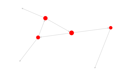
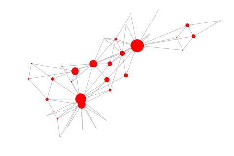
Centrality is also a whole world on its own. If you wish to visualize the betweenness centrality you can use something like:
cent = nx.centrality.betweenness_centrality(gr)
nx.draw(gr, node_size=[v * 1500 for v in cent.values()], edge_color='silver')
Getting the connected components of a graph:
nx.is_connected(gr.to_undirected())
comps = nx.components.connected_components(gr.to_undirected())
for c in comps:
	print(c)
Clique
A clique is a complete subgraph of a particular size. Large, dense subgraphs are useful for example in the analysis of protein-protein interaction graphs, specifically in the prediction of protein complexes.
def show_clique(graph, k = 4):
	'''
		Draws the first clique of the specified size.
	'''
	cliques = list(nx.algorithms.find_cliques(graph))
	kclique = [clq for clq in cliques if len(clq) == k]
	if len(kclique)>0:
		print(kclique[0])
		cols = ["red" if i in kclique[0] else "white" for i in graph.nodes() ]
		nx.draw(graph, with_labels=True, node_color= cols, edge_color="silver")
		return nx.subgraph(graph, kclique[0])
	else:
		print("No clique of size %s."%k)
		return nx.Graph()
Taking the Barabasi graph above and checking for isomorphism with the complete graph of the same size we can check that the found result is indeed a clique of the requested size.
subg = show_clique(ba,5)
nx.is_isomorphic(subg, nx.complete_graph(5))
red = nx.random_lobster(100, 0.9, 0.9) nx.draw(ba)
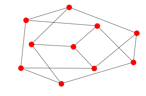
petersen = nx.petersen_graph()
nx.draw(petersen)
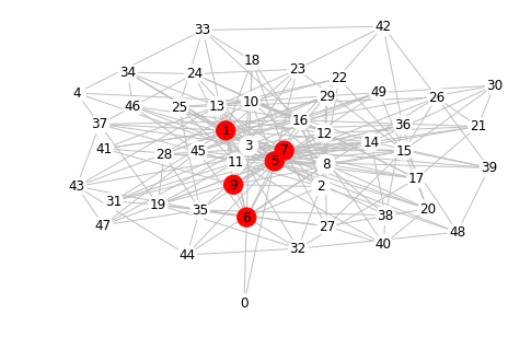
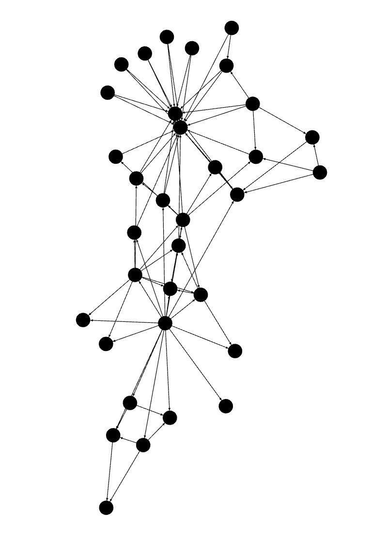
G=nx.karate_club_graph()
cent = nx.centrality.betweenness_centrality(G)
nx.draw(G, node_size=[v * 1500 for v in cent.values()], edge_color='silver')
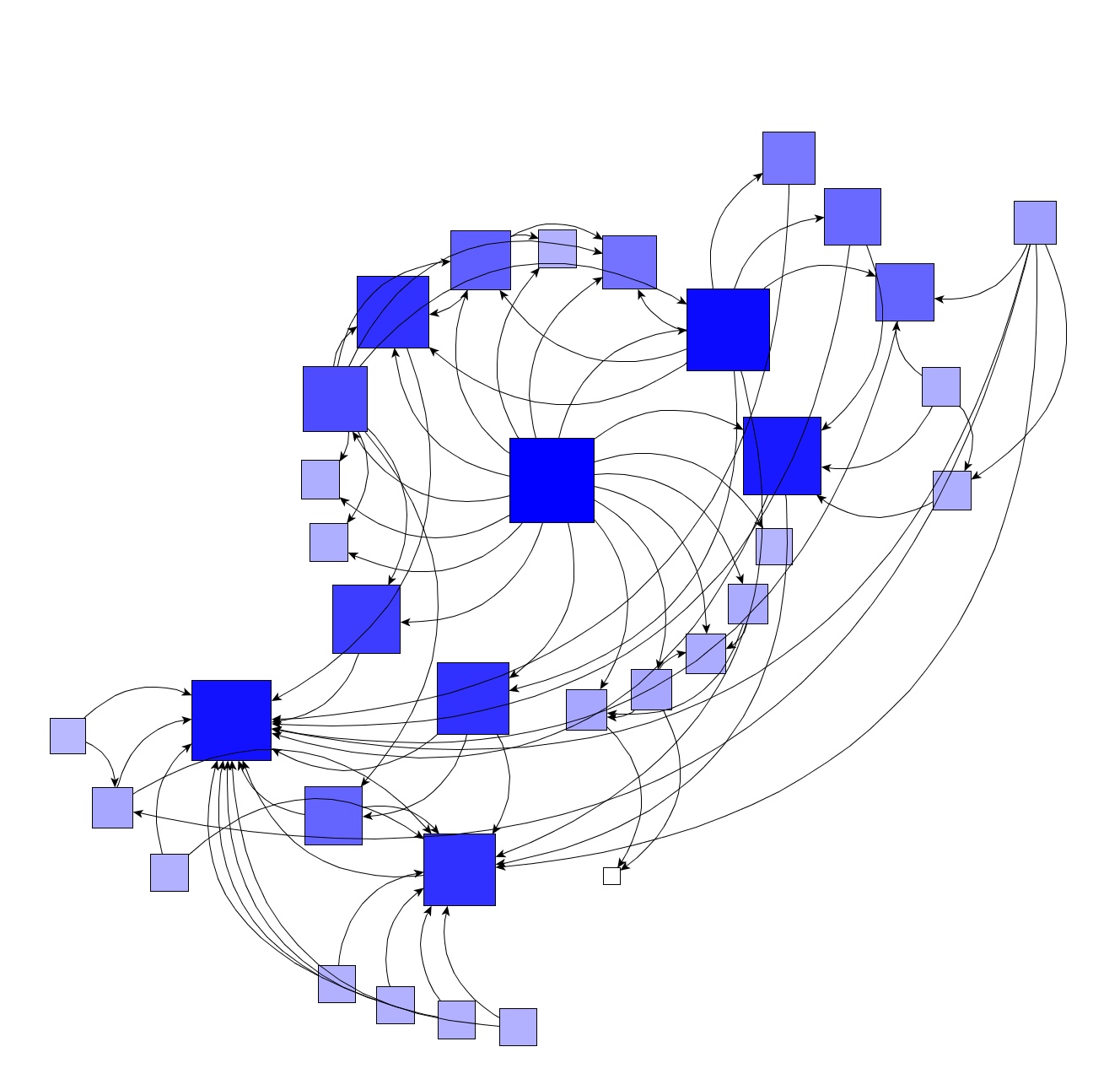
Graph visualization
As described above, if you want pretty images you should use packages outside NetworkX. The dot and GraphML formats are standards and saving a graph to a particular format is really easy.
For example, here we save the karate-club to GraphML and used yEd to layout things together with a centrality resizing of the nodes.
G=nx.karate_club_graph()
nx.write_graphml(G, "./karate.graphml")
For Gephi you can use the GML format:
nx.write_gml(G, "./karate.gml")
Get and set data
In the context of machine learning and real-world data graphs it’s important that nodes and edges carry data. The way it works in NetworkX can be a bit tricky, so let’s make it clear here how it functions.
Node get/set goes like this:
G = nx.Graph()
G.add_node(12, payload = {'id': 44, 'name': 'Swa' })
print(G.nodes[12]['payload'])
print(G.nodes[12]['payload']['name'])
One can also set the data after the node is added:
G = nx.Graph()
G.add_node(12)
nx.set_node_attributes(G, {12:{'payload':{'id': 44, 'name': 'Swa' }}})
print(G.nodes[12]['payload'])
print(G.nodes[12]['payload']['name'])
Edge get/set is like so:
G = nx.Graph()
G.add_edge(12,15, payload={'label': 'stuff'})
print(G.get_edge_data(12,15))
print(G.get_edge_data(12,15)['payload']['label'])
One can also set the data after the edge is added:
G = nx.Graph()
G.add_edge(12,15)
nx.set_edge_attributes(G, {(12,15): {'payload':{'label': 'stuff'}}})
print(G.get_edge_data(12,15))
print(G.get_edge_data(12,15)['payload']['label'])
Pandas
The library has support for import/export from/to Pandas dataframes. This exchange, however, applies to edges and not to nodes. The row of a frame are used to define an edge and if you want to use a frame for nodes or both, you are on your own. It’s not difficult though, let’s take a graph and turn it into a frame.
g = nx.barabasi_albert_graph(50, 5)
# set a weight on the edges
for e in g.edges:
	nx.set_edge_attributes(g, {e: {'weight':faker.random.random()}})
for n in g.nodes:
	nx.set_node_attributes(g, {n: {"feature": {"firstName": faker.first_name(), "lastName": faker.last_name()}}})
You can now use the to_pandas_edgeList method but this will only output the weights besides the edge definitions:
nx.to_pandas_edgelist(g)
source	target	weight
0	0	1	0.140079
1	0	2	0.986347
2	0	3	0.932105
3	0	4	0.673917
4	0	5	0.395162
...	...	...	...
220	37	46	0.233217
221	39	43	0.264401
222	39	44	0.112617
223	39	45	0.408708
224	39	48	0.782268
import pandas as pd
import copy
node_dic = {id:g.nodes[id]["feature"] for id in g.nodes} # easy acces to the nodes
rows = [] # the array we'll give to Pandas
for e in g.edges:
    row = copy.copy(node_dic[e[0]])
    row["sourceId"] = e[0]
    row["targetId"] = e[1]
    row["weight"] = g.edges[e]["weight"]
    rows.append(row)
df = pd.DataFrame(rows)
df
| FIRSTNAME | LASTNAME | SOURCEID | TARGETID | WEIGHT | |
|---|---|---|---|---|---|
| 0 | Rebecca | Griffin | 0 | 5 | 0.021629 |
| 1 | Rebecca | Griffin | 0 | 6 | 0.294875 |
| 2 | Rebecca | Griffin | 0 | 7 | 0.967585 |
| 3 | Rebecca | Griffin | 0 | 8 | 0.553814 |
| 4 | Rebecca | Griffin | 0 | 9 | 0.531532 |
| … | … | … | … | … | … |
| 220 | Tyler | Morris | 40 | 43 | 0.313282 |
| 221 | Mary | Bolton | 41 | 42 | 0.930995 |
| 222 | Colton | Hernandez | 42 | 48 | 0.380596 |
| 223 | Michael | Moreno | 43 | 46 | 0.236164 |
| 224 | Mary | Morris | 45 | 47 | 0.213095 |
Note that you need this denormalization of the node data because you actually need two datasets to describe a graph in a normalized fashion.
StellarGraph
The StellarGraph library can import directly from NetworkX and Pandas via the static StellarGraph.from_networkx method.
One important thing to note here is that the features on a node as defined above will not work because the framework expects numbers and not strings or dictionaries. If you do take care of this (one-hot encoding and all that) then this following will do:
from stellargraph import StellarGraph
gs = StellarGraph.from_networkx(g,
	edge_type_default = "relation",
	node_type_default="person",
	node_features = "feature",
	edge_weight_attr = "weight")
print(gs.info())
StellarGraph: Undirected multigraph
 Nodes: 50, Edges: 225
 Node types:
  default: [50]
    Features: none
    Edge types: default-default->default
 Edge types:
    default-default->default: [225]
Alternatives
If NetworkX does not contain what you are looking for or if you need more performance, the iGraph packageis a good alternative and has bindings for C, R and Mathematica while NetworkX is only working with Python. Another very fast package is the Graph-Tool framework with heaps of features.
Beyond these standalone packages there are also plenty of frameworks integrating with various databases and, of course, the Apache universe. Each graph database has its own graph analytics stack and you should spend some time investigating this space especially because it scales beyond what the standalone packages can.
Finally, graph analytics can also go into terabytes via out-of-memory algorithms, Apache Spark and GPU processing to name a few. The RapidsAI framework is a great solutions with the cuGraph API running on GPU and is largely compatible with the NetworkX API.